performance_tests.py
SOURCE: performance_tests.py
This code will help us generate and analyze performance runs for VASP. The docstrings below should clearly explain what is happening in the code. Here we will focus on how to use it from the command line.
Generating Directories
First we will need a seed POSCAR and INCAR. We will take the example of LaNiO3. The POSCAR is here:
t
3.825747
1 0 0
0 1 0
0 0 1
1 1 3
d
0.5 0.5 0.5 La
0.0 0.0 0.0 Ni
0.5 0.0 0.0 O
0.0 0.5 0.0 O
0.0 0.0 0.5 O
Now we will need whatever common set of parameters that are to be used in the INCAR. This could be left totally blank. However, in this case I will assume that we want a particular ISMEAR:
ISMEAR=-5
Now we will need a configuration file called “config” in our directory. It should look like this:
supa=[1,2,3,4]
cutoff=[200,250,300,350,400,450]
kpts=[8,10,12,14,16]
struct=poscar
incar=incar
The first variable will define how many multiples of the primitive cell that we have. As indicated, we will loop over 1-4 times the number of atoms in the primitive cell. Second, we will give the range of cutoffs. Third, we give the range of kpoints, and at the moment they have to be the same in all directions. We could change this later. Finally, we give the names for the seed INCAR and POSCAR that are used to generate the run. We can now generate the runs as follows:
$ performance_tests.py -generate
$ ls
run_cut0250_k12_mult001  run_cut0300_k16_mult004  run_cut0400_k12_mult003
run_cut0250_k12_mult002  run_cut0350_k08_mult001  run_cut0400_k12_mult004
run_cut0250_k12_mult003  run_cut0350_k08_mult002  run_cut0400_k14_mult001
etc..
# If you like you can queue everything up with roborun.py and boomerang.py...
$ roborun.py 'pwd;boomerang.py -queue'
Extracting Data
After running the directories you generated, you will want to harvest the data. Alternatively, you may have run your own suite of runs and want to analyze the data. You can do this using the data extraction procedure. I extract most of the keys things you would want to know, but it would be easy to add more by looking at the docstrings below. So we just need to run the code and give the prefix of the directories plus a proper regular expression to match all of the directories.
$ performance_tests.py gather=run_*
The default behavior is to output the raw data to the screen. This could be analyzed in a spreadsheet easily. However, the code also outputs a sqlite database which can easily be queried for whatever you want. The default name for the database is vasp_timing_data.db. Using these tools it should be pretty trivial to create benchmarks under a wide variety of conditions on a lot of different hardware.
Let us practice extracting timing from the database. Please remind yourself of the basics of SQL from our previous group meeting intro. You can familiarize yourself with the SQL language on wikipedia. In this script we will first yank out all of the different cutoffs that we explored, then you will loop through them and yank out the number of kpoints for that run and the total time. I then plot these using gracey, though you may prefer to use matplotlib or something else.
from gracey import plot
import sqlite3 as lite
import sys


con = lite.connect('vasp_timing_data.db')
cur = con.cursor()

# get the cuttoffs...
cur.execute("SELECT cut FROM vasp_timing_data ")
cuttoff = sorted(list(set([s[0] for s in cur.fetchall()])))

# now let us plot time vs nk for each cuttoff...
aa=plot()
for ii in cuttoff:
  cur.execute("SELECT nk,total_time FROM vasp_timing_data WHERE cut=%s ORDER BY nk"%ii)
  rows = cur.fetchall()
  aa.function(rows)

aa.quickin("""leg=%s"""%(str([str(int(s))+'eV' for s in cuttoff]).replace(" ","").replace("'","")))
aa.quickin("""
yl=seconds xl=irreducible__kpoints  pr=800,600 xr=15,125 xt=10
lw=2 ll=0.2,0.8 lcs=2
t=LaNiO3__run__times
st=Run__on__i3770__-__Primitive__unit__cell
""")
aa.show()
aa.picname='../figures/fig_timing_k_cut'
aa.show('EPS')
aa.quickin('pr=1200,900')
aa.show('PNG')
Now let us see what we have found:

Timing for LaNiO3. Here we plot the time as a function of the irreducible kpoints
for different values of the plane wave cutoff.
EPS
Comparing different processors
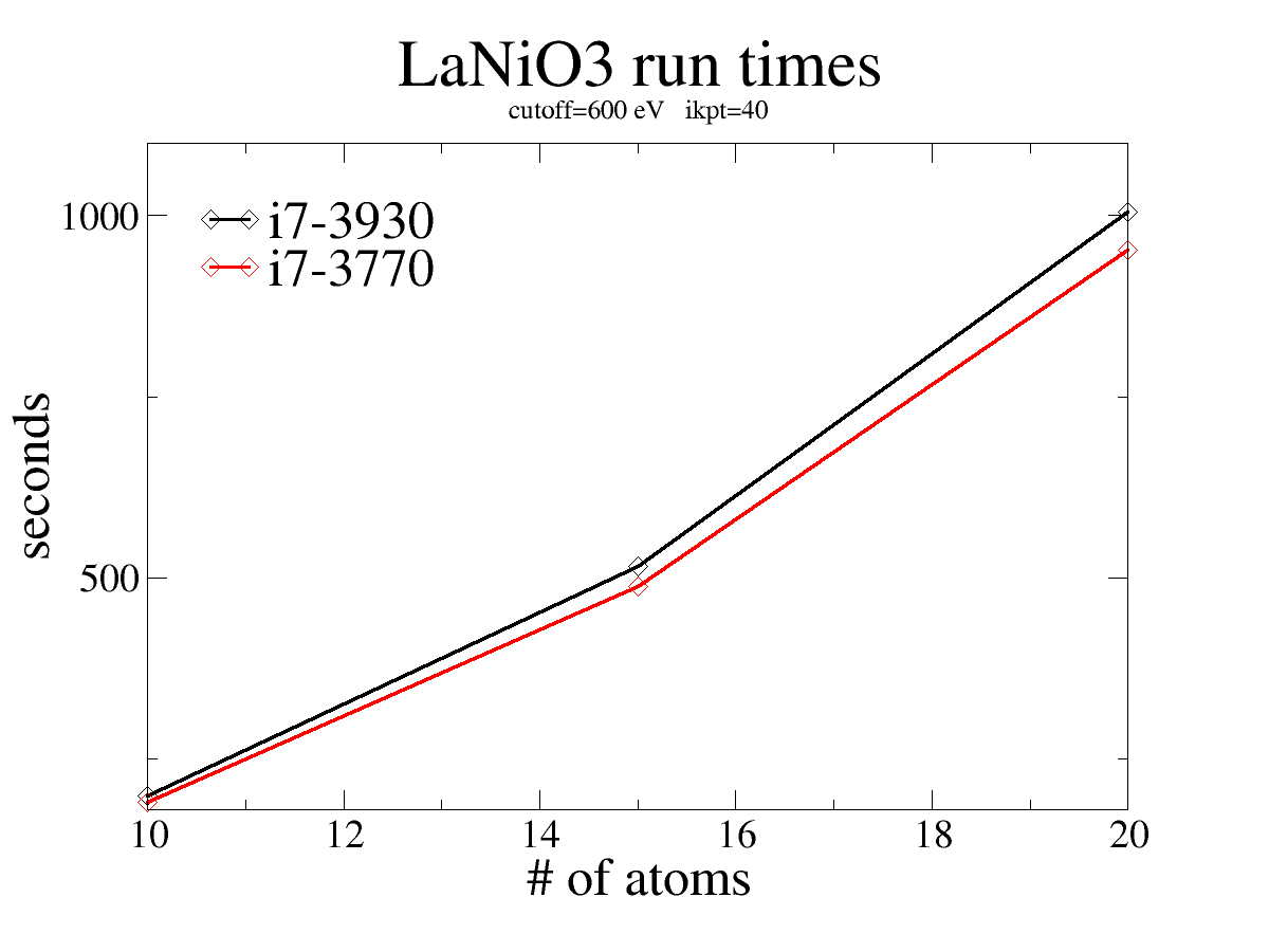
i7-3930 vs i7-3770. Here we plot the time as a function of the number of atoms. Results were very comparable for other kpt/cutoff slices. The 3930 appears to be consistently 5-7% slower.