Hamiltonian

Hamiltonian classes are used to manipulate electron and phonon Hamiltonians to compute various properties including band structure and density of states. We also included a model Hamiltonian class allowing us to work with simple theory models.

Here we demonstrate the usage of Hamiltonian classes with simple models.

Model Hamiltonian

Model Hamiltonian class serves as a container for simple Hamiltonians. For example, we can create a 1-dimensional Hamiltonian with nearest neighbor hopping as follows:

>>> hamiltonian_dict = {
        ( 0, 0, 0): [[0.00]],
        ( 1, 0, 0): [[0.25]],
        (-1, 0, 0): [[0.25]],
    }
>>> ham = ModelHamiltonian()
>>> ham.set_hamiltonian(np.array(list(hamiltonian_dict.keys())), np.array(list(hamiltonian_dict.values())))
>>> ham.tpoints
array([[ 0,  0,  0],
       [ 1,  0,  0],
       [-1,  0,  0]])
>>> ham.hamiltonian_matrices
array([[[0.  ]],

       [[0.25]],

       [[0.25]]])

We can use this Hamiltonian in our 1D Hubbard model to study its electronic band structure.

Electron Hamiltonian - 1D Hubbard Model

First, we create a CrystalFTG object with the structure of a 1D crystal of 1 atom per unit cell, and we will be studying the electrons in the \(s\) orbital.

>>> vec = np.identity(3)
>>> atoms = {"H": np.array([[0, 0, 0],])}
>>> orbitals = "s"
>>> supa = np.identity(3, dtype=int)
>>> structure = CrystalFTG(vec=vec, atoms=atoms, orbitals=orbitals, supa=supa)

With the Hamiltonian created in Model Hamiltonian, we can construct the electron Hamiltonian class and compute the Fermi energy (\(E_f=0~eV\)) and density of states (shown in Fig. 3).

>>> mesh = np.diag([2000, 1, 1])
>>> eham = ElectronHamiltonian(structure=structure, pg="C1", mesh=mesh, nelect=1)
>>> eham.set_hamiltonian(ham)
>>> eham.set_hamiltonian_from_mesh()
>>> print(eham.get_fermi_energy())
0.0
>>> dos = eham.compute_DOS(1000)
>>> plt.plot(eham._dos_bins - eham.get_fermi_energy(), dos)
>>> plt.ylabel("DOS".format(eham.units))
>>> plt.xlabel(r"$E - E_f$ (eV)".format(eham.units))

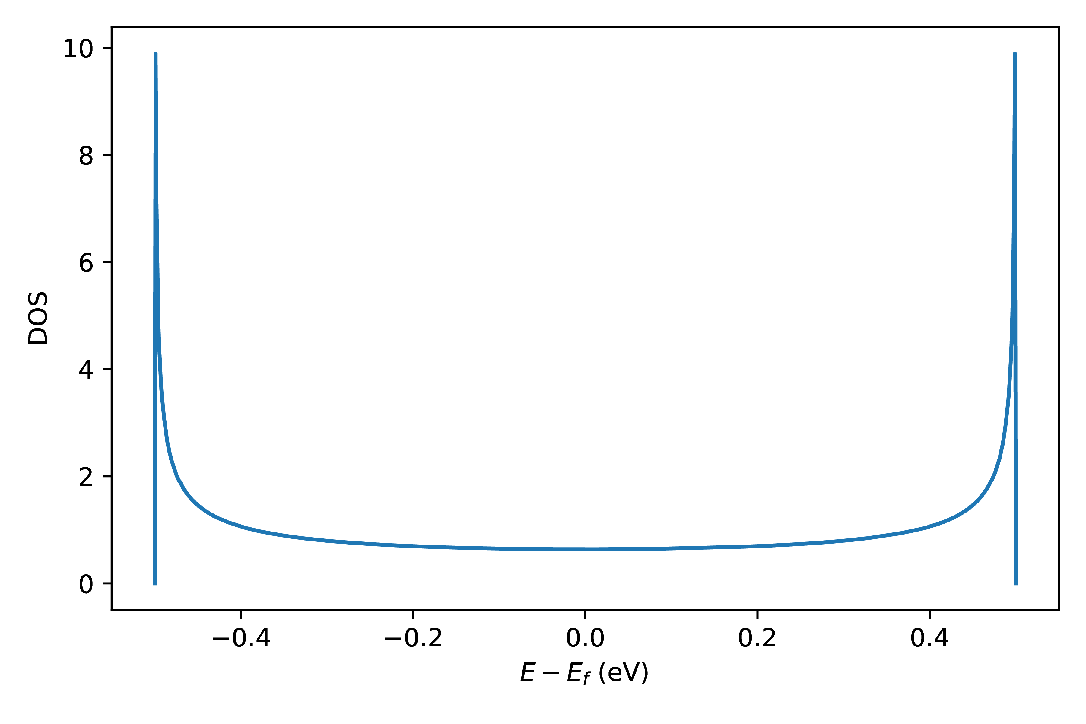
Fig. 3 Density of states of 1D Hubbard module.

Phonon Hamiltonian - Square Lattice

For the purpose of simplicity, we refer to square lattice to demonstrate the usage of phonon Hamiltonian. First we create a CrystalFTG object of a square lattice:

>>> vec = np.diag([1, 1, 60])
>>> atoms = {"C": np.array([[0, 0, 0],])}
>>> orbitals = "p_z"
>>> supa = np.identity(3, dtype=int)
>>> structure = CrystalFTG(vec=vec, atoms=atoms, orbitals=orbitals, supa=supa)

Then we can construct a model Hamiltonian of force constants with only the nearest neighbor forces.

>>> gamma = 1
>>> force_constants = {
        ( 0,  0, 0): [[ 4 * gamma]],
        ( 1,  0, 0): [[-1 * gamma]],
        (-1,  0, 0): [[-1 * gamma]],
        ( 0,  1, 0): [[-1 * gamma]],
        ( 0, -1, 0): [[-1 * gamma]],
    }
>>> ham = ModelHamiltonian()
>>> ham.set_hamiltonian(np.array(list(force_constants.keys())), np.array(list(force_constants.values())))

With the above structure and Hamiltonian, we can construct the phonon Hamiltonian object and compute the phonon band structure of the square lattice.

mesh = np.diag([1, 1, 1])
pham = PhononHamiltonian(structure=structure, pg="C1", mesh=mesh)
pham.set_hamiltonian(ham)
pham.set_hamiltonian_from_mesh()

However, in order to compute the band structure, we need to setup the \(\textbf{q}\)-point path. Here we choose the compute the band along the path from \(\vec{\Gamma}=\left(0,0\right)\) to \(\vec{X}=\left(\frac{1}{2},0\right)\), \(\vec{R}=\left(\frac{1}{2},\frac{1}{2}\right)\) and back to \(\vec{\Gamma}\).

>>> vertices = parse_array("""
        0 0 0
        1/2 0 0
        1/2 1/2 0
        0 0 0
    """, dtype=float)
>>> vertices_names = [
        r"$\Gamma$",
        "X",
        "R",
        r"$\Gamma$",
    ]
>>> kpath = KPath(
        vertices=vertices,
        vertices_names=vertices_names,
        npoints=101,
    )
>>> kpath.set_kpath()

Once the path is setup, we can compute the \(\textbf{q}\)-points along the path and plot the phonon spectrum as shown in Fig. 4.

>>> pham.set_hamiltonian_at_kpoints(kpath.kpoints)
>>> plt.close()
>>> plt.plot(kpath.kpoints_distances, pham._eigenvalues[:, 0])
>>> for i in range(len(kpath.vertices_distances)):
        plt.plot(
            [kpath.vertices_distances[i], kpath.vertices_distances[i]],
            [0, np.max(pham._eigenvalues) * 1.05],
            c="gray",
            ls="-",
            lw=1
        )
>>> plt.ylim(0, np.max(pham._eigenvalues) * 1.05)
>>> plt.xticks(kpath.vertices_distances.tolist(), kpath.vertices_names)
>>> plt.ylabel("Frequencies ({})".format(pham.units))

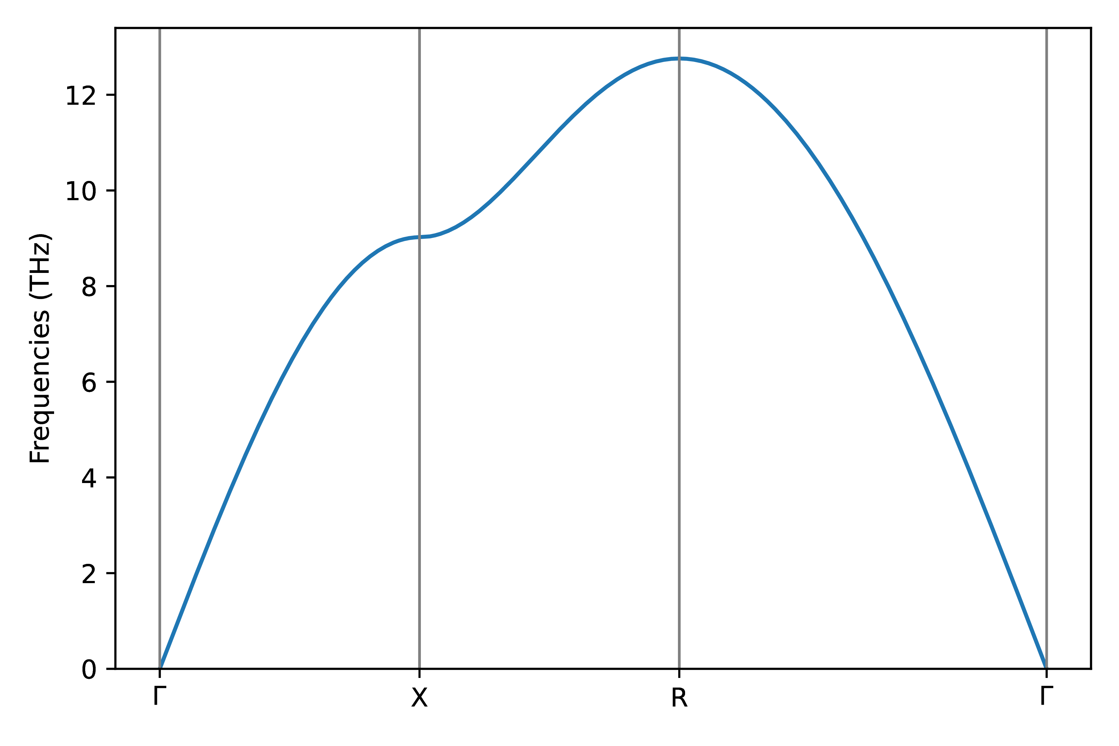
Fig. 4 Phonon band structure of square lattice.