
Phonons and their interactions
Computing phonons and their interactions is one of the main feature we developed in this thesis. Here we will break down the workflow in the key features including finite displacements, symmetry analysis, lone irreducible derivatives approach (LID), bundled irreducible derivatives approach (BID), hierarchical supercell bundled irreducible derivatives approach (HS-BID) and phonon linewidth and thermal conductivity.
In this section we will mainly use NaCl as an example material (see structure illustration in Fig. 5), for the finite displacements demonstration, symmetry analysis, and phonon calculations with LID, BID and HS-BID approaches. We will demonstrate phonon linewidth and conductivity predicted with phonon interaction coefficients using \(\textrm{ThO}_2\).
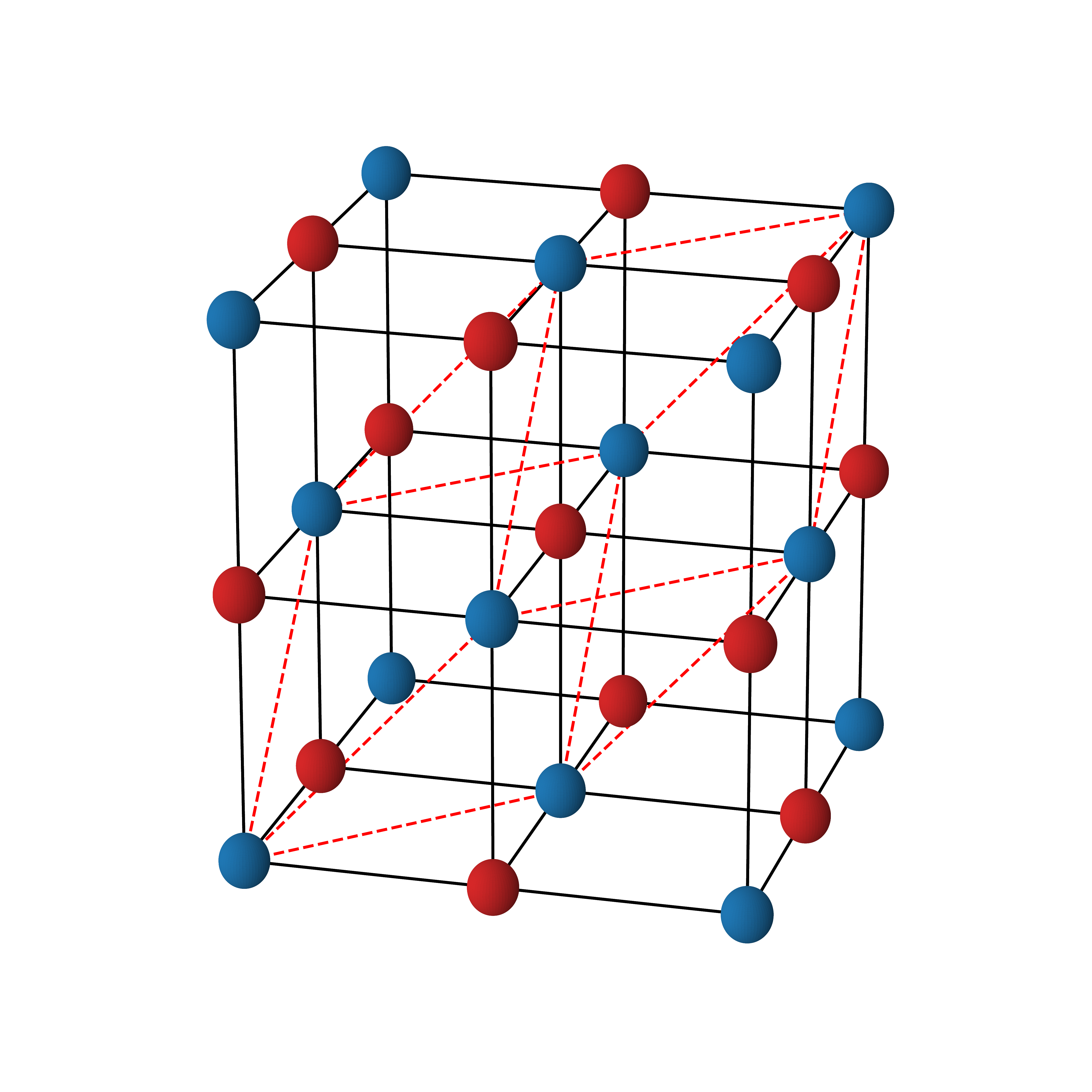
Fig. 5 A schematic of the structure of the cubic unit cell (i.e. \(\hat{S}_{BZ}=\hat{S}_{C}\) where \(\hat{S}_{C}\) is defined below) of rock salt NaCl, where the blue spheres represent the Na atoms, and the red spheres the Cl atoms. The red dashed lines enclose the primitive unit cell (i.e. \(\hat{S}_{BZ}=\hat{1}\)).
Finite Displacements
Finite displacements method takes derivatives of a function with respect to atomic displacements using finite difference approach. As we can see from the flowchart that illustrates the workflow of our finite displacements approach in Fig. 6, we begin by constructing the finite displacement stencils of the measurement. With the displacement amplitudes \(\Delta\) we can find the unique jobs that need computed from a first principle approach, where each job simply represent the structure of the material of interest at a certain supercell that includes some displacements and sometimes even strain. We emphasize that we adopt a database centered approach and we store all the jobs inside a database. The input files of the first principle calculations are created from the database and the results from the calculations, including energy, forces, etc., are also parsed from the output of the first principle calculations and stored into the database. These results will then be served from the database to compute the finite displacement derivatives.
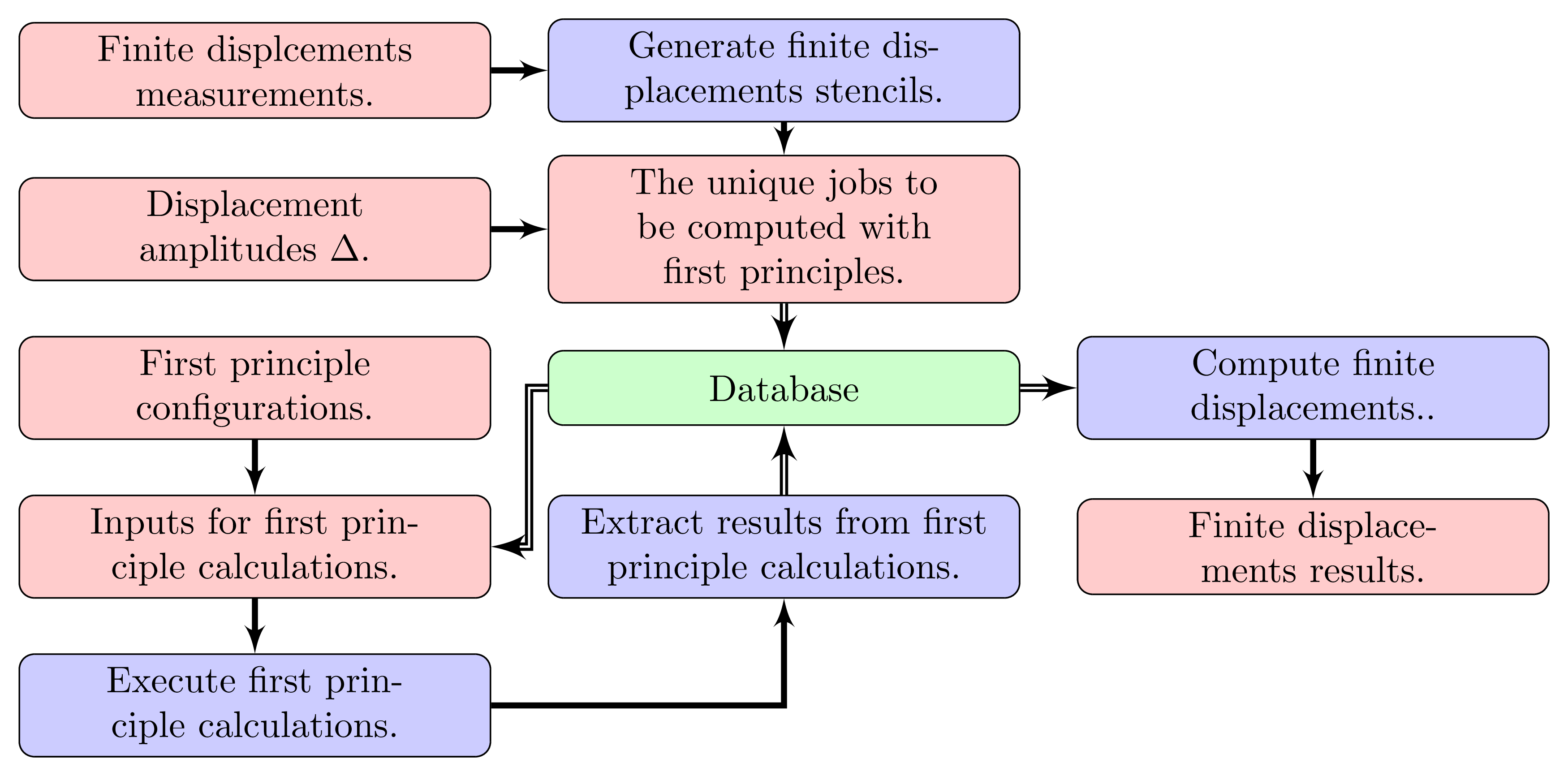
Fig. 6 Flowchart illustrating the workflow of the finite displacements implementation, where red boxes represent quantities, blue boxes represent operations and green box database. Single-lined arrows represent the direction of the workflow and double-lined arrows the direction of data in and out of the database.
Since the finite displacements method is simply the finite difference with respect to the nuclei displacements, we first present the FiniteDifference class that houses all the abstract finite difference functionalities, including construction of stencils and steps, where a step is a point \((x_1^{\prime},\cdots, x_n^{\prime})\) at which the target function \(f(x_1,\cdots, x_n)\) of the finite difference is evaluated at in order to compute the finite difference derivative. Additionally, unique steps reduces redundancy considering computing finite difference at multiple \(\Delta\) at the same time.
>>> fdiff = FiniteDifference(order=(2, 1))
>>> fdiff.set_delta(np.arange(0.01, 0.03, 0.01))
>>> fdiff.set_steps()
>>> fdiff._stencils
array([[ 2,  1],
       [ 2, -1],
       [ 0,  1],
       [ 0, -1],
       [-2,  1],
       [-2, -1]])
>>> fdiff.uniq_steps
array([[-0.04, -0.02],
       [-0.04,  0.02],
       [-0.02, -0.01],
       [-0.02,  0.01],
       [ 0.  , -0.02],
       [ 0.  , -0.01],
       [ 0.  ,  0.01],
       [ 0.  ,  0.02],
       [ 0.02, -0.01],
       [ 0.02,  0.01],
       [ 0.04, -0.02],
       [ 0.04,  0.02]])
With these unique steps and the displacements basis to take the derivatives of, the FiniteDisplacements class is able compute displacements needed to be applied to the structure.
>>> supa = np.identity(3, dtype=int) * 2
>>> fd = FiniteDisplacements(
        structure=structure,
        supa=supa,
        fdtype="c",
        tol=1.0E-6,
        )
>>> displacements = np.zeros((2, ) + fd.supercell.positions.shape)
>>> displacements[0][0, 0] = 1
>>> displacements[1][1, 0] = 1
>>> fd.set_displacement_vectors(dispvecs=displacements, displabels=[1, 2])
>>> fd.set_delta([0.01, 0.02])
Although we normally would store the jobs into a database and compute first principles from there, in this demonstration we can directly create the input files for the first principle calculations. Here we use VASP to compute the energy and forces at the displacements, and we can create the jobs from the displacements and the supercell matrix for VASP to compute.
>>> fd.set_jobs()
>>> root_directory = "fd_runs"
>>> dft_engine = "vasp"
>>> job_handler = ComputeJobSeries(
      structure=fd.supercell,
      root_directory=root_directory,
      compute_engine=dft_engine,
      config_path=None,
      )
>>> fd.create_jobs(
      job_handler=job_handler,
    )
Additionally, we can also use strained finite displacements class to compute the derivatives of a function with respect to strain and displacements at the same time. In this following demonstration, we compute the second order derivative of \(\varepsilon_{xx}\) strain of energy.
>>> supa = np.identity(structure.dim, dtype=int)
>>> sfd = StrainedFiniteDisplacements(
      structure=structure,
      supa=supa,
      )
>>> sfd.set_strain(strain=[e_xx, ], strain_orders=(2, ))
>>> strain_delta = np.arange(0.005, 0.03, 0.005)
>>> sfd.set_strain_delta(strain_delta)
>>> sfd.set_finite_difference()
Here we have the first principle calculation already finished and stored in a database, we can retrieve the energy from the database and compute the finite displacements.
>>> sfd.set_jobs(skip_zero=False)
>>> job_handler = JobsDB(
      structure=structure,
      root_directory="nacl_sfd",
      db_path="nacl_sfd/database.db",
      db_type="sqlite"
      )
>>> job_handler.set_table("strain")
>>> sfd.create_jobs(
      job_handler=job_handler,
      dry_run=True,
      )
>>> sfd.set_raw_results(
      source=job_handler,
      data_type="energy"
      )
>>> sfd.compute_finite_displacements()
Since the strained finite displacements calculations are computed with multiple deltas and with central finite difference, we can compute the quadratic error tail (see Fig. 7) and extrapolate to \(\delta \to 0\), and finally obtain the second order derivative of \(\varepsilon_{xx}\): \(\partial^2 V / \partial \varepsilon_{xx}^2 = 13.75 eV\).
>>> result, xcoef, pick, penalty = get_errortail(
      deltas=strain_delta,
      values=sfd.fd_result.reshape((-1, 1)),
      fdtype="c",
      pick_min=3,
      pick_max=5,
      separate_complex=False,
      return_xcoef=True,
      return_pick=True,
      return_penalty=True,
      )
>>> result[0]
13.750108012806797
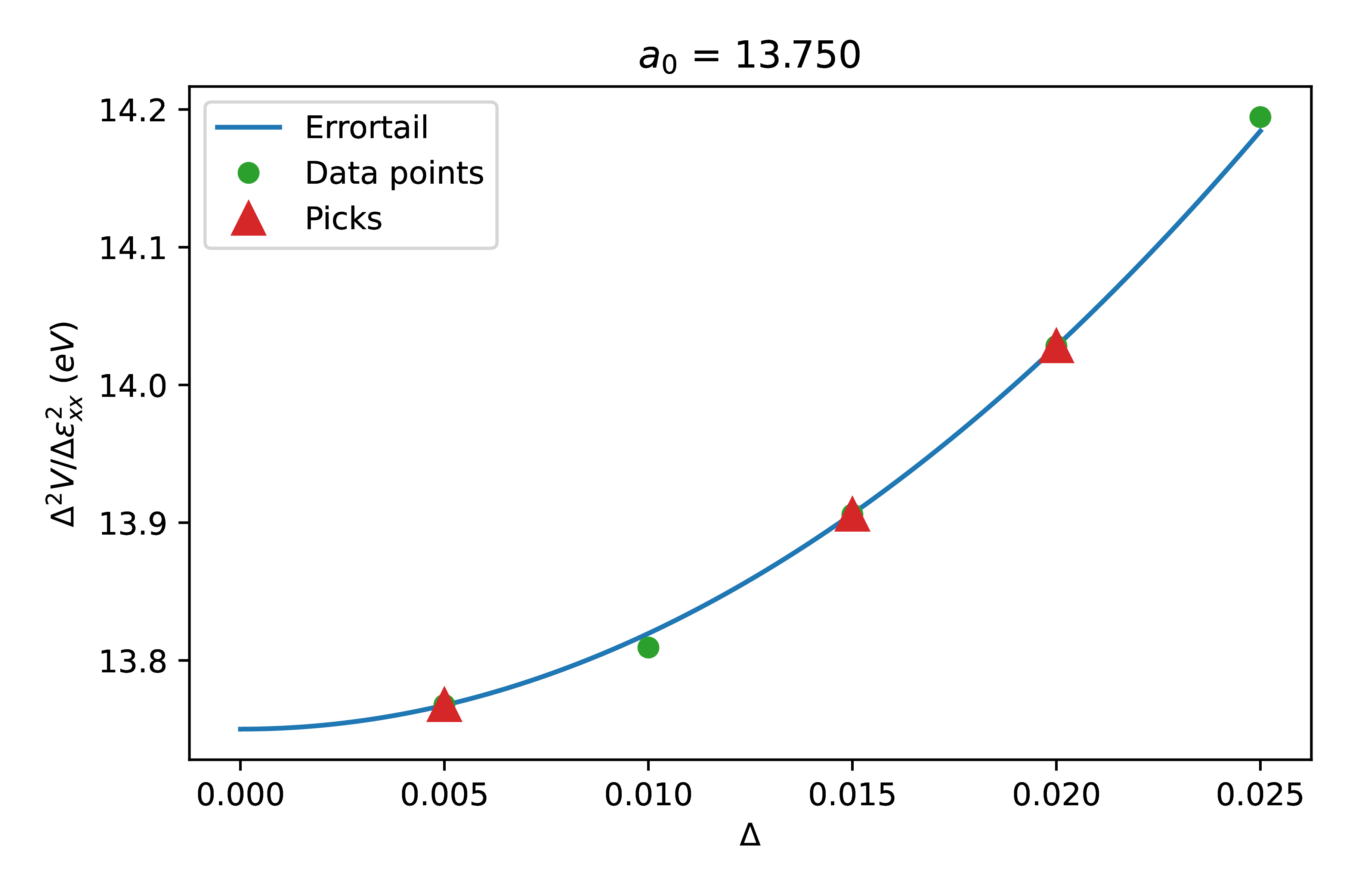
Fig. 7 Quadratic error tail of the finite difference calculation \(\Delta^2 V / \Delta \varepsilon_{xx}^2\), where the green circles and the red triangles are the \(\Delta\) at which the finite displacements are computed and the blue line is the fitted quadratic error tail. The red triangles are the points picked when fitting the error tail.
Phonon Interaction Symmetry Analysis
The group theory behind the symmetry analysis of phonon interactions can be found in the paper, and the workflow is illustrated in the flowchart in Fig. 8. First we need the information for the symmetry analysis, which includes the crystal structure, the space group of the crystal, the FTG \(\hat{S}_{BZ}\) (i.e. a supercell) and the order \(\mathcal{N}\) of the interaction. Subsequently, we can find the irreducible \(Q\)-points \(\tilde{Q}_{IBZ}\) with the aforementioned information, and then we can find the irreducible representations of the nuclei displacements at each \(\textbf{q} \in Q\). Then the symmetric direct products can be constructed for find the irreducible derivatives allowed by group theory for each \(Q \in \tilde{Q}_{IBZ}\), and the irreducible basis of the identity representations in the symmetric direct products determine the coefficients on how to populate the analytic dynamic tensors in the symmetrized basis. We can write out the phonon Hamiltonian in terms of the irreducible derivatives by multiplying the analytic dynamic tensors with their respective displacements basis. Additionally, sparse tensors can implemented for analytic dynamic tensors to increase space efficiency.
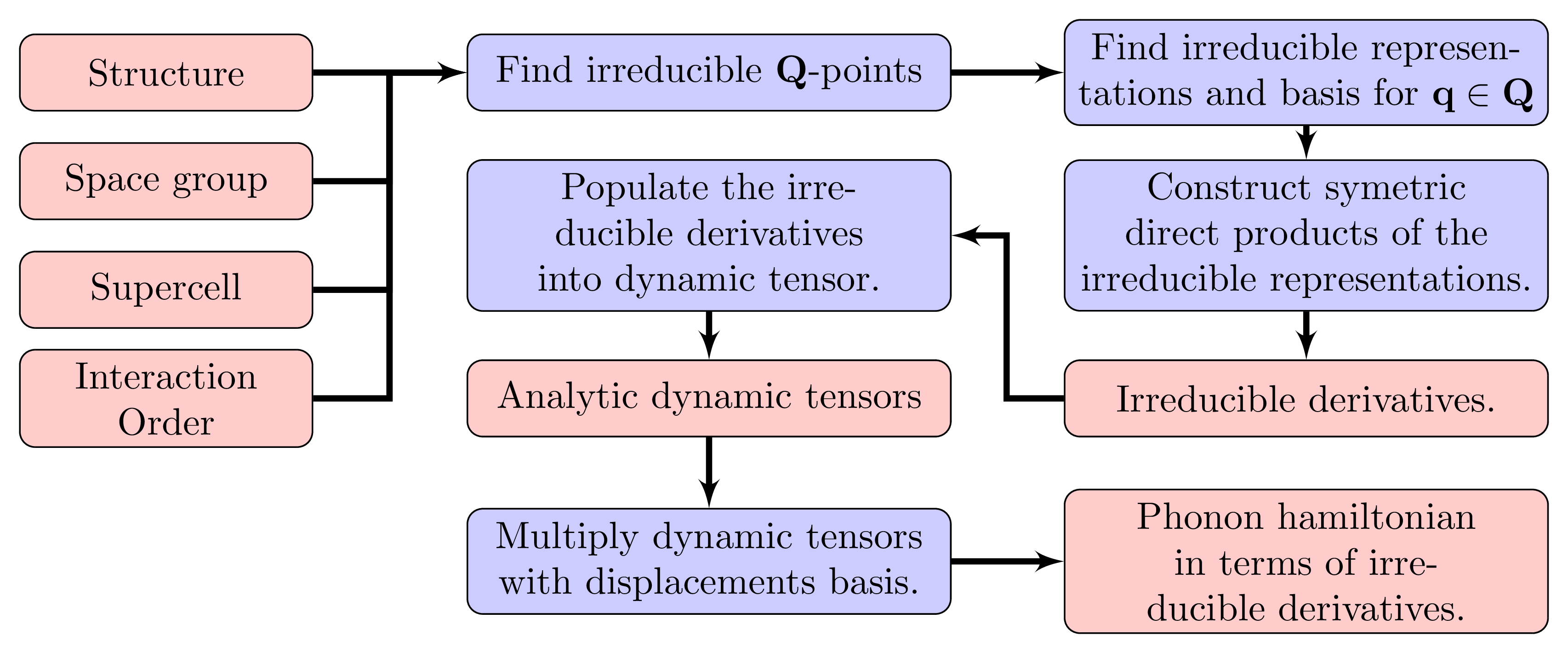
Fig. 8 Flowchart illustrating the workflow of phonon interaction symmetry analysis we implemented, where red boxes represent quantities, blue boxes represent operations and green box database. Single-lined arrows represent the direction of the workflow.
The rock salt structure is used for demonstration. We can start with building an analytic dynamic tensor for a given \(Q\)-point. For example, at second order we can build the analytic tensor for \(Q = \left[L_x, L_x\right]\), and we can see that the first irreducible derivative in this \(Q\) contributes to a \(3\time3\) submatrix of the analytic dynamic tensor in the naive basis:
>>> Qpoint = parse_array("1/2 0 0; 1/2 0 0", dtype=Fraction)
>>> Qpoint
[[Fraction(1, 2), Fraction(0, 1), Fraction(0, 1)],
 [Fraction(1, 2), Fraction(0, 1), Fraction(0, 1)]]
>>> lgadt = LittleGroupADT(
        structure=structure,
        pg="Oh",
        Qpoint=Qpoint)
>>> lgadt.set_qpoint_displacement_rep()
>>> lgadt.set_irreducible_derivatives()
>>> lgadt.set_vectorized_tensor()
>>> lgadt.irreducible_derivative_names
[((((Fraction(1, 2), Fraction(0, 1), Fraction(0, 1)), ('A1g', 0)),
   ((Fraction(1, 2), Fraction(0, 1), Fraction(0, 1)), ('A1g', 0))),
  ('A1g', 0)),
 ((((Fraction(1, 2), Fraction(0, 1), Fraction(0, 1)), ('Eg', 0)),
   ((Fraction(1, 2), Fraction(0, 1), Fraction(0, 1)), ('Eg', 0))),
  ('A1g', 0)),
 ((((Fraction(1, 2), Fraction(0, 1), Fraction(0, 1)), ('A2u', 0)),
   ((Fraction(1, 2), Fraction(0, 1), Fraction(0, 1)), ('A2u', 0))),
  ('A1g', 0)),
 ((((Fraction(1, 2), Fraction(0, 1), Fraction(0, 1)), ('Eu', 0)),
   ((Fraction(1, 2), Fraction(0, 1), Fraction(0, 1)), ('Eu', 0))),
  ('A1g', 0))]
>>> print(lgadt.vectorized_tensor[:, :, 0].real)
[[ 0.          0.          0.          0.          0.          0.        ]
 [ 0.          0.          0.          0.          0.          0.        ]
 [ 0.          0.          0.          0.          0.          0.        ]
 [ 0.          0.          0.          0.33333333 -0.33333333 -0.33333333]
 [ 0.          0.          0.         -0.33333333  0.33333333  0.33333333]
 [ 0.          0.          0.         -0.33333333  0.33333333  0.33333333]]
% We can also construct the analytic dynamic tensor at third order for \(Q = \left[\Gamma, L_x, L_x\right]\):
>>> Qpoint = parse_array("0 0 0; 1/2 0 0; 1/2 0 0", dtype=Fraction)
>>> Qpoint
[[Fraction(0, 1), Fraction(0, 1), Fraction(0, 1)],
 [Fraction(1, 2), Fraction(0, 1), Fraction(0, 1)],
 [Fraction(1, 2), Fraction(0, 1), Fraction(0, 1)]]
>>> lgadt = LittleGroupADT(
        structure=structure,
        pg="Oh",
        Qpoint=Qpoint)
>>> lgadt.set_qpoint_displacement_rep()
>>> lgadt.set_irreducible_derivatives()
>>> lgadt.set_vectorized_tensor()
>>> lgadt.irreducible_derivative_names
[((((Fraction(0, 1), Fraction(0, 1), Fraction(0, 1)), ('A2u', 0)),
   ((Fraction(1, 2), Fraction(0, 1), Fraction(0, 1)), ('A1g', 0)),
   ((Fraction(1, 2), Fraction(0, 1), Fraction(0, 1)), ('A2u', 0))),
  ('A1g', 0)),
 ((((Fraction(0, 1), Fraction(0, 1), Fraction(0, 1)), ('A2u', 0)),
   ((Fraction(1, 2), Fraction(0, 1), Fraction(0, 1)), ('Eg', 0)),
   ((Fraction(1, 2), Fraction(0, 1), Fraction(0, 1)), ('Eu', 0))),
  ('A1g', 0)),
 ((((Fraction(0, 1), Fraction(0, 1), Fraction(0, 1)), ('Eu', 0)),
   ((Fraction(1, 2), Fraction(0, 1), Fraction(0, 1)), ('A1g', 0)),
   ((Fraction(1, 2), Fraction(0, 1), Fraction(0, 1)), ('Eu', 0))),
  ('A1g', 0)),
 ((((Fraction(0, 1), Fraction(0, 1), Fraction(0, 1)), ('Eu', 0)),
   ((Fraction(1, 2), Fraction(0, 1), Fraction(0, 1)), ('A2u', 0)),
   ((Fraction(1, 2), Fraction(0, 1), Fraction(0, 1)), ('Eg', 0))),
  ('A1g', 0)),
 ((((Fraction(0, 1), Fraction(0, 1), Fraction(0, 1)), ('Eu', 0)),
   ((Fraction(1, 2), Fraction(0, 1), Fraction(0, 1)), ('Eg', 0)),
   ((Fraction(1, 2), Fraction(0, 1), Fraction(0, 1)), ('Eu', 0))),
  ('A1g', 0))]
Second, we construct the analytic tensors for a given FTG at a given order. For example, for the FTG \(\hat{S}_{BZ}=2\hat{1}\), we can build analytic dynamic tensors with the AnalyticTensors class and find the irreducible derivatives allowed by group theory.
>>> supa = np.diag([2, 2, 2])
>>> at = AnalyticTensors(
        structure=structure,
        supa=supa,
        order=2,
        pg="Oh",
    )
>>> at.set_ADT(
        little_group=True,
        verbose=True,
    )
Computing ADT for Qpoint: ((0, 0, 0), (0, 0, 0))
Computing ADT for Qpoint: ((1/2, 0, 0), (1/2, 0, 0))
Computing ADT for Qpoint: ((1/2, 1/2, 0), (1/2, 1/2, 0))
Summarize irreducible derivatives.
Compute vectorized tensors.
>>> for irreducible_derivative in at.irreducible_derivative_names:
>>>     print(tuple_to_str(irreducible_derivative))
((((0, 0, 0), (T1u, 0)), ((0, 0, 0), (T1u, 0))), (A1g, 0))
((((1/2, 0, 0), (A1g, 0)), ((1/2, 0, 0), (A1g, 0))), (A1g, 0))
((((1/2, 0, 0), (Eg, 0)), ((1/2, 0, 0), (Eg, 0))), (A1g, 0))
((((1/2, 0, 0), (A2u, 0)), ((1/2, 0, 0), (A2u, 0))), (A1g, 0))
((((1/2, 0, 0), (Eu, 0)), ((1/2, 0, 0), (Eu, 0))), (A1g, 0))
((((1/2, 1/2, 0), (A2u, 0)), ((1/2, 1/2, 0), (A2u, 0))), (A1g, 0))
((((1/2, 1/2, 0), (A2u, 0)), ((1/2, 1/2, 0), (A2u, 1))), (A1g, 0))
((((1/2, 1/2, 0), (A2u, 1)), ((1/2, 1/2, 0), (A2u, 1))), (A1g, 0))
((((1/2, 1/2, 0), (Eu, 0)), ((1/2, 1/2, 0), (Eu, 0))), (A1g, 0))
((((1/2, 1/2, 0), (Eu, 0)), ((1/2, 1/2, 0), (Eu, 1))), (A1g, 0))
((((1/2, 1/2, 0), (Eu, 1)), ((1/2, 1/2, 0), (Eu, 1))), (A1g, 0))
Furthermore, with the analytic tensors of the FTG, we are able to perform more complicated analysis on phonon interactions. One of them is using chain rule derivatives to compute the transformation matrices of arbitrary displacements for BID approach.
For the purpose of simplicity, we use the FTG \(\hat{S}_{BZ}=\hat{S}[C]\) as an example to compute the chain rule matrix of the displacement along \(x\)-axis of the first {Na} atom with the ChainruleDerivatives class, and from the resulting chain rule matrix we can see that such simple displacement probed multiple irreducible derivatives in the FTG \(\hat{S}_{BZ}=\hat{S}[C]\).
>>> supa = np.ones((3, 3), dtype=int) - 2 * np.identity(3, dtype=int)
>>> chainrule =  ChainruleDerivatives(
        structure=structure,
        supa=supa,
        order=2,
        pg='Oh')
>>> chainrule.set_ADT(verbose=True)
Computing ADT for Qpoint: ((0, 0, 0), (0, 0, 0))
Computing ADT for Qpoint: ((1/2, 1/2, 0), (1/2, 1/2, 0))
Summarize irreducible derivatives.
Compute vectorized tensors.
>>> chainrule.set_basis()
>>> displacements = np.zeros((1, chainrule.order - 1, chainrule.supercell.natoms, chainrule.supercell.dim))
>>> displacements[0, 0, 0, 0] = 1
>>> matrix = chainrule.compute_chainrule(displacements)
>>> matrix.reshape((-1, chainrule.n_irreducible_derivatives)).real
array([[ 0.25,  0.  ,  0.  ,  0.  ,  0.  ,  0.  ,  0.  ],
       [-0.  ,  0.  ,  0.  ,  0.  ,  0.  ,  0.  ,  0.  ],
       [ 0.  ,  0.  ,  0.  ,  0.  ,  0.  ,  0.  ,  0.  ],
       [-0.25,  0.  ,  0.  ,  0.  ,  0.  ,  0.  ,  0.  ],
       ...,
       [ 0.  ,  0.  ,  0.5 ,  0.  ,  0.  ,  0.  ,  0.  ],
       [ 0.  ,  0.  ,  0.  ,  0.  ,  0.  , -0.  ,  0.  ],
       [ 0.  ,  0.  ,  0.  ,  0.  ,  0.  , -0.  , -0.  ]])
Lone Irreducible Derivatives Approach
The LID approach performs symmetry analysis for phonons and phonon interactions at each \(\mathcal{Q}\)-point individually, and find displacements to perturb each irreducible derivative separately.
The LID approach tries to compute one irreducible derivative or as few irreducible derivatives as possible with a single measurement. As shown in the flowchart in Fig. 9, we begin with the analytic dynamic tensors obtained with the workflow described in phonon interaction symmetry analysis. We can find the symmetrized displacements basis sets the probes the irreducible derivatives as separately as possible, but these displacements are generally complex since they carry a phase in the Fourier series. Therefore, we need to apply a similarity transformation and transform those complex displacements to displacements that are purely real (see the paper for details). We can compute the finite displacements with the workflow described in finite displacements, after we obtained the measurements in the real space, and extrapolate quadratic error tails for the \(\Delta \to 0\) results. Finally, we can solve for the irreducible derivatives with the finite displacements derivatives extrapolated from the error tail.
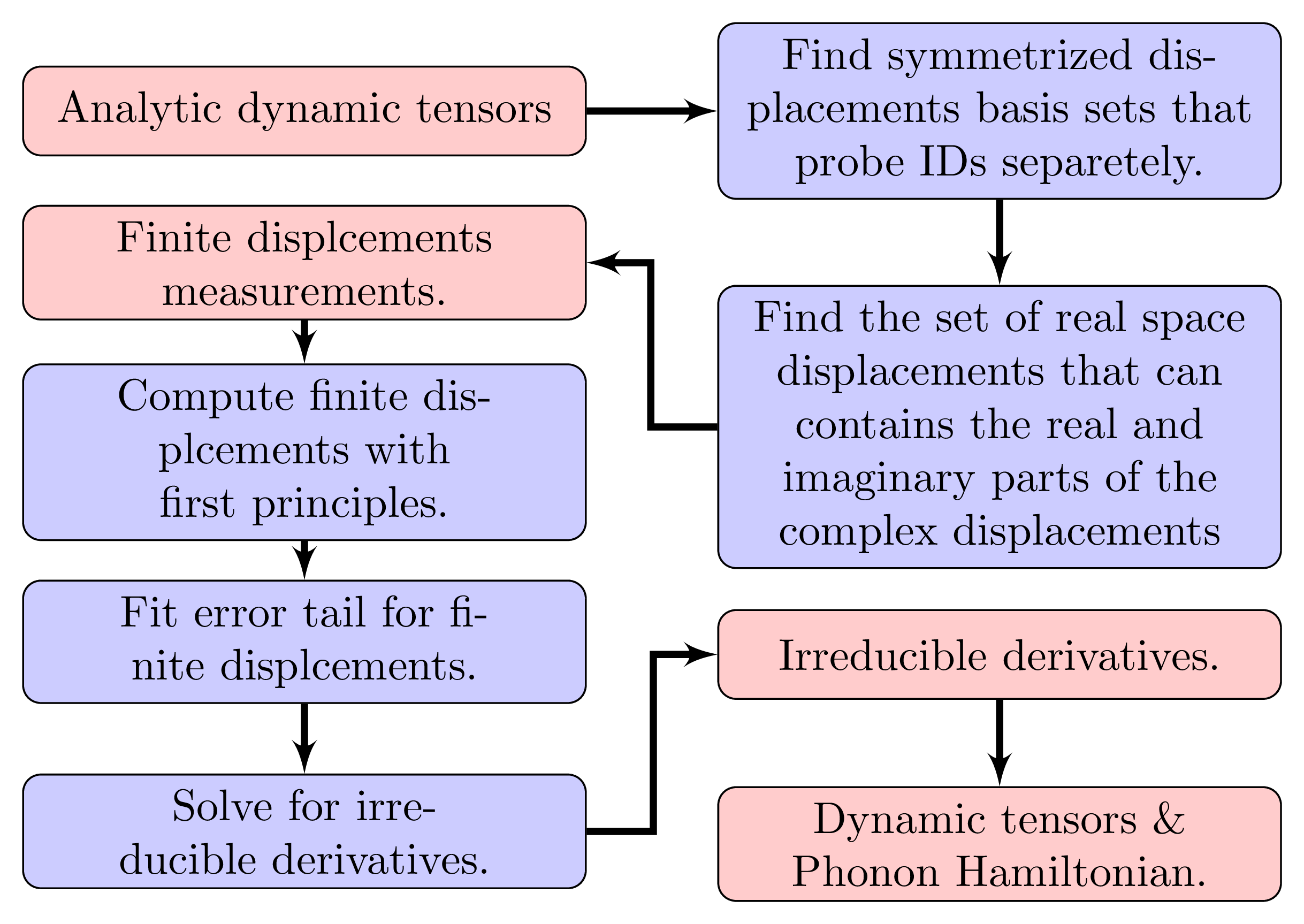
Fig. 9 Flowchart illustrating the workflow of LID approach, where red boxes represent quantities, blue boxes represent operations and green box database. Single-lined arrows represent the direction of the workflow.
We demonstrate the workflow of the LID approach with the rock salt structure, at second order and \(\hat{S}_{BZ}=2\hat{1}\). Additionally, we will be using central finite difference on forces from the first principle calculations so that we only need first order finite displacements derivatives. First we can construct the LIDMesh object with said configurations:
>>> ORDER = 2
>>> PG = "Oh"
>>> MESH = np.diag([2, 2, 2])
>>> lid_mesh = LIDMesh(
      structure=structure,
      supa=MESH,
      order=ORDER,
      pg=PG,
      )
>>> lid_mesh.set_lid()
Setting up LID for Qpoint: ((0, 0, 0), (0, 0, 0))
Setting up LID for Qpoint: ((1/2, 0, 0), (1/2, 0, 0))
Setting up LID for Qpoint: ((1/2, 1/2, 0), (1/2, 1/2, 0))
Then we can create the finite displacements jobs that first principle calculations need to be executed at. We will store the jobs into a database since we are using a database centric approach.
>>> job_handler= JobsDB(
      structure=structure,
      root_directory=".",
      db_path="nacl_lid/database.db",
      db_type="sqlite",
      )
>>> job_handler.set_table("lid_phonon")
>>> DELTA = np.arange(0.02, 0.21, 0.02)
>>> lid_mesh.create_jobs(
        job_handler=job_handler,
        deltas=DELTA,
        append=True,
        dry_run=True,
        )
Once we finished the first principles calculations, and store the results back into the database, we can compute the finite displacements, extrapolate the quadratic error tail and finally compute the irreducible derivatives and the dynamic tensors from the finite displacements results.
>>> lid_mesh.set_results(
        job_handler=job_handler,
        data_type="forces",
        )
>>> lid_mesh.set_errortail_results(
        pick_min=3,
        pick_max=5,
        separate_complex=True,
        )
>>> dynamic_tensors = lid_mesh.get_dynamic_tensors()
>>> for i in range(len(lid_mesh.QpointsN.irreducible_Qpoints)):
        print(tuple_to_str(lid_mesh.QpointsN.irreducible_Qpoints[i]))
        print(dynamic_tensors.real[i])
((0, 0, 0), (0, 0, 0))
[[ 1.2142316  0.         0.        -1.2142316  0.         0.       ]
 [ 0.         1.2142316  0.         0.        -1.2142316  0.       ]
 [ 0.         0.         1.2142316  0.         0.        -1.2142316]
 [-1.2142316  0.         0.         1.2142316  0.         0.       ]
 [ 0.        -1.2142316  0.         0.         1.2142316  0.       ]
 [ 0.         0.        -1.2142316  0.         0.         1.2142316]]
((1/2, 0, 0), (1/2, 0, 0))
[[ 2.18334962 -0.80283112 -0.80283112  0.          0.          0.        ]
 [-0.80283112  2.18334962  0.80283112  0.          0.          0.        ]
 [-0.80283112  0.80283112  2.18334962  0.          0.          0.        ]
 [ 0.          0.          0.          2.30355673 -0.76809942 -0.76809942]
 [ 0.          0.          0.         -0.76809942  2.30355673  0.76809942]
 [ 0.          0.          0.         -0.76809942  0.76809942  2.30355673]]
((1/2, 1/2, 0), (1/2, 1/2, 0))
[[ 1.47829446  0.          0.          1.02011023  0.          0.        ]
 [ 0.          1.47829446  0.          0.          1.02011023  0.        ]
 [ 0.          0.          1.99846289  0.          0.         -0.59315421]
 [ 1.02011023  0.          0.          2.09150467  0.          0.        ]
 [ 0.          1.02011023  0.          0.          2.09150467  0.        ]
 [ 0.          0.         -0.59315421  0.          0.          3.44754191]]
We can compute the phonon band structure with LO-TO splitting with the computed dynamic tensors, dielectric tensor and born effective charges, using Fourier interpolation. (Note that the above demonstration used \(\hat{S}_{BZ}=2\hat{1}\) for simplicity, but the Fig. 10 used \(\hat{S}_{BZ}=4\hat{1}\) as the denser FTG contains for information at a relatively cheap computational cost).
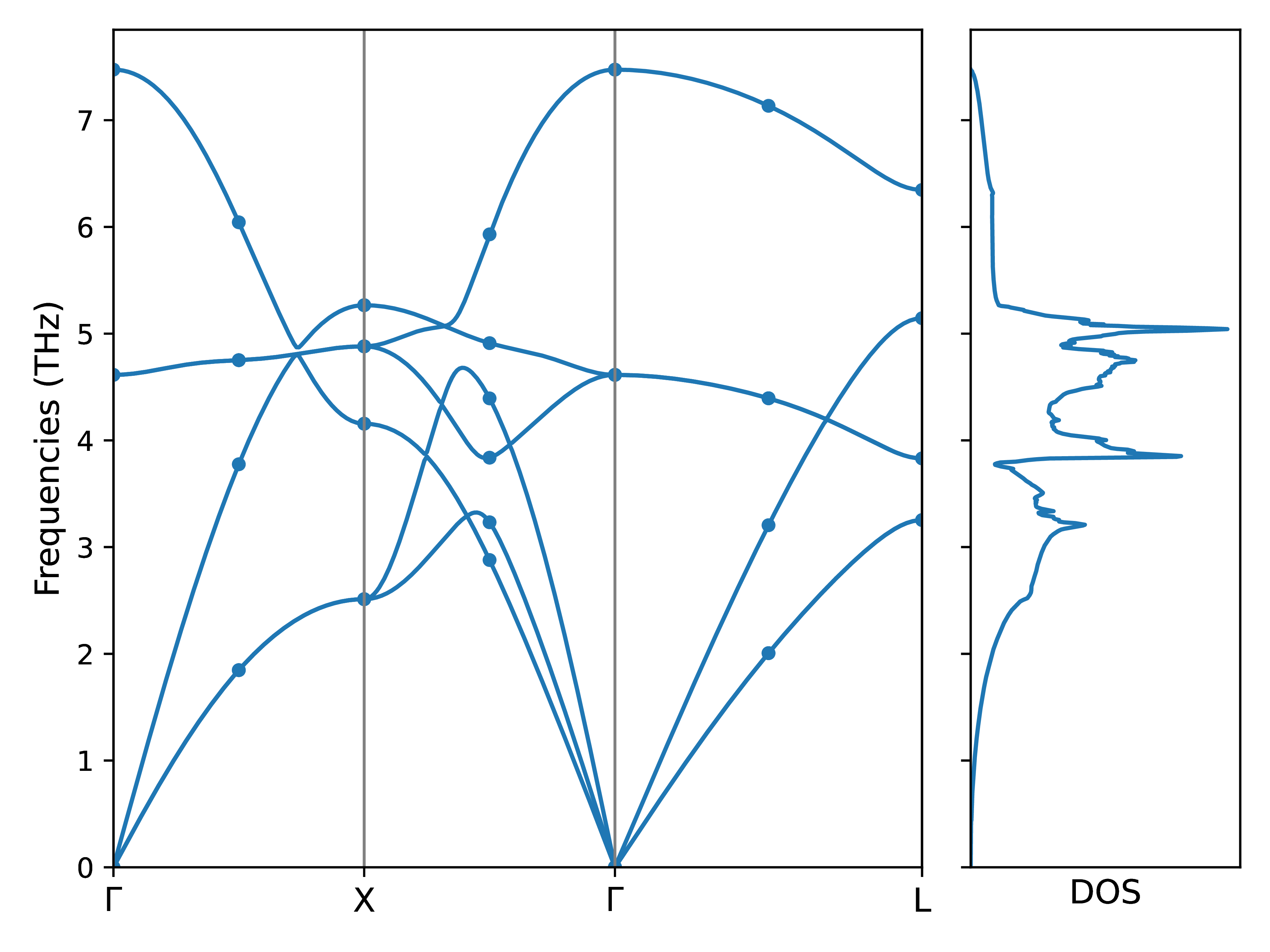
Fig. 10 Phonon and DOS of NaCl with FTG 4:math:hat{1} including LO-TO splitting.
Furthermore, we can also construct the LID object for a single \(Q\)-point if we are only studying that \(Q\)-point, and follow the similar workflow as above to create first principle calculations and compute the finite displacements from the results.
%TODO
>>> Qpoint = np.array(parse_array("1/2 0 0; 1/2 0 0", dtype=Fraction))
>>> lid = LoneID_FP(
        structure=structure,
        Qpoint=Qpoint,
        pg=PG,
        )
>>> lid.set_analytic_tensor()
>>> lid.set_displacements_basis()
>>> lid.set_displacements()
>>> lid.set_realspace_displacements()
Bundled Irreducible Derivatives Approach
label{sec:si:phonon:bid}
Both SS-BID and HS-BID approaches try to compute all irreducible derivatives at a given FTG and order with as few measurements as possible. The workflow of SS-BID is illustrated in the flowchart in Fig. 11. First we estimate the minimum number of measurements needed N with dividing the total number of irreducible derivatives with the rank of the chain rule matrix of a single measurement. Then we generate N measurements and if the chain rule matrix of the measurements is not full rank, we increment N by 1 until resulting chain rule matrix is full rank. In practice we try a few measurement sets at each N to make sure we can’t reach full rank with N measurements. Once we find the minimum number of measurements, we compute the finite displacements, fit the quadratic error tail and solve for the irreducible derivatives. Finally, we can compute the dynamic tensors and phonon Hamiltonian with the irreducible derivatives. With the HS-BID approach, we find the hierarchical supercells for the irreducible \(Q\)-points with a greedy algorithm, and execute SS-BID at each supercell, while counting for the irreducible derivatives at the smaller supercells as known derivatives.
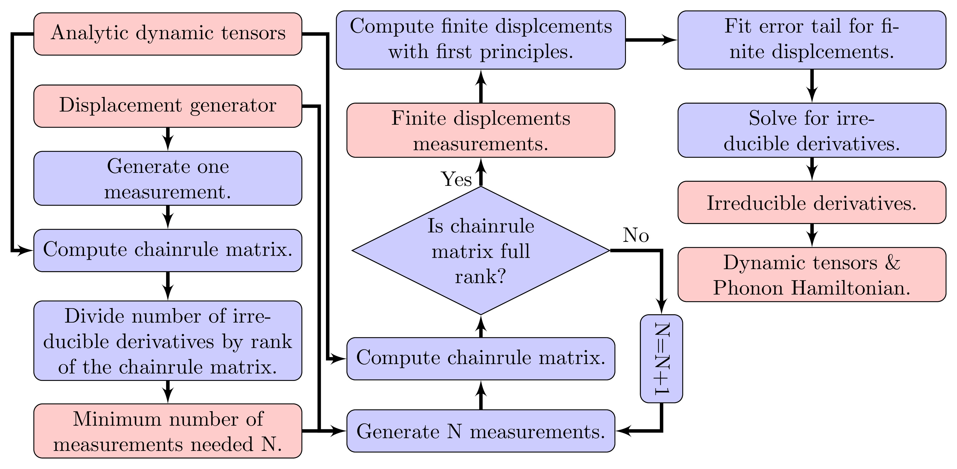
Fig. 11 Flowchart illustrating the workflow of BID approach, where red boxes represent quantities, blue boxes represent operations and green box database. Single-lined arrows represent the direction of the workflow.
Here we use \(\hat{S}_{BZ}=2\hat{1}\) to demonstrate the workflow of SS-BID and HS-BID approaches. First, we can construct the BID object with the same configurations as those used for the LID object in lone irreducible derivatives approach.
>>> ORDER = 2
>>> PG = "Oh"
>>> MESH = np.diag([2, 2, 2])
>>> bid = BID(
      structure=structure,
      supa=MESH,
      order=ORDER,
      pg=PG,
      )
>>> bid.set_chainrule_derivatives(verbose=True)
>>> bid._set_displacement_generator()
>>> bid.find_measurements(verbose=True)
Computing ADT for Qpoint: ((0, 0, 0), (0, 0, 0))
Computing ADT for Qpoint: ((1/2, 0, 0), (1/2, 0, 0))
Computing ADT for Qpoint: ((1/2, 1/2, 0), (1/2, 1/2, 0))
Summarize irreducible derivatives.
Compute vectorized tensors.
Number of unknowns:  11
Rank of single measurements:  11
Estimated number of measurements:  1
Then we can create the finite displacements jobs and store them in a database.
>>> job_handler= JobsDB(
      structure=structure,
      root_directory=ROOT_DIR,
      db_path="nacl_hsbid/database.db",
      db_type="sqlite",
      )
>>> job_handler.set_table("bid_phonon")
>>> DELTA = np.arange(0.02, 0.21, 0.02)
>>> bid.create_jobs(
        job_handler=job_handler,
        deltas=DELTA,
        append=True,
        )
After the first principle calculations are finished, we can retrieve the results and compute irreducible derivatives with finite displacements.
>>> bid.set_results(
        job_handler=job_handler,
        data_type="forces",
        )
>>> bid.set_errortail_results(
        pick_min=3,
        pick_max=5,
        separate_complex=True,
        output="out_errortail.hdf5",
        )
>>> bid.compute_irreducible_derivatives()
However, with the SS-BID approach all of the irreducible derivatives are computed from a single FTG, which shown by our minimum supercell multiplicity equation derived in the paper, is very inefficient. And the SS-BID approach is not able to utilize the irreducible derivatives already computed from a smaller FTG and we have to perform redundant computations, further decreasing the efficiency.
Thus, the hierarchical supercell BID approach is needed to address these problems. HS-BID uses a greedy algorithm to find the minimum number of supercells to satisfy that each irreducible derivative can be computed in the smallest possible supercell the derivative fits in.
We can construct a HS-BID object with the same configurations as the BID object above.
>>> hsbid = HSBID(
      structure=structure,
      supa=MESH,
      order=ORDER,
      pg=PG,
      )
>>> hsbid.set_chainrule_derivatives(verbose=True)
>>> hsbid.set_hsbid()
>>> hsbid.find_measurements(verbose=True)
Computing ADT for Qpoint: ((0, 0, 0), (0, 0, 0))
Computing ADT for Qpoint: ((1/2, 0, 0), (1/2, 0, 0))
Computing ADT for Qpoint: ((1/2, 1/2, 0), (1/2, 1/2, 0))
Summarize irreducible derivatives.
Compute vectorized tensors.
Find measurements for supercell # 0
Number of unknowns:  1
Rank of single measurements:  1
Estimated number of measurements:  1
Find measurements for supercell # 1
Number of unknowns:  4
Rank of single measurements:  4
Estimated number of measurements:  1
Find measurements for supercell # 2
Number of unknowns:  6
Rank of single measurements:  5
Estimated number of measurements:  2
And create the finite displacements jobs with the same job_handler object to store them into the database.
>>> hsbid.create_jobs(
        job_handler=job_handler,
        deltas=DELTA,
        append=True,
        )
Here we can use the finished first principle results stored in the database to compute finite displacements and solve for the irreducible derivatives and dynamic tensors.
>>> hsbid.set_results(
        job_handler=job_handler,
        data_type="forces",
        )
>>> hsbid.set_errortail_results(
        pick_min=3,
        pick_max=5,
        separate_complex=True,
        )
>>> hsbid.compute_irreducible_derivatives()
>>> dynamic_tensors = hsbid.get_dynamic_tensors()
>>> for i in range(len(hsbid._chainrule.QpointsN.irreducible_Qpoints)):
>>>     print(tuple_to_str(hsbid._chainrule.QpointsN.irreducible_Qpoints[i]))
>>>     print(dynamic_tensors[hsbid._chainrule.QpointsN.irreducible_Qpoints_Qind].real[i])
((0, 0, 0), (0, 0, 0))
[[ 1.2163185  0.         0.        -1.2163185  0.         0.       ]
 [ 0.         1.2163185  0.         0.        -1.2163185  0.       ]
 [ 0.         0.         1.2163185  0.         0.        -1.2163185]
 [-1.2163185  0.         0.         1.2163185  0.         0.       ]
 [ 0.        -1.2163185  0.         0.         1.2163185  0.       ]
 [ 0.         0.        -1.2163185  0.         0.         1.2163185]]
((1/2, 0, 0), (1/2, 0, 0))
[[ 2.18264725 -0.80163822 -0.80163822  0.          0.          0.        ]
 [-0.80163822  2.18264725  0.80163822  0.          0.          0.        ]
 [-0.80163822  0.80163822  2.18264725  0.          0.          0.        ]
 [ 0.          0.          0.          2.30057778 -0.76845191 -0.76845191]
 [ 0.          0.          0.         -0.76845191  2.30057778  0.76845191]
 [ 0.          0.          0.         -0.76845191  0.76845191  2.30057778]]
((1/2, 1/2, 0), (1/2, 1/2, 0))
[[ 1.47854869  0.          0.          1.0212613   0.          0.        ]
 [ 0.          1.47854869  0.          0.          1.0212613   0.        ]
 [ 0.          0.          1.99804315  0.          0.         -0.59932048]
 [ 1.0212613   0.          0.          2.09450795  0.          0.        ]
 [ 0.          1.0212613   0.          0.          2.09450795  0.        ]
 [ 0.          0.         -0.59932048  0.          0.          3.44972342]]
Same as lone irreducible derivatives approach, we can compute phonon band structure and density of states with LO-TO splitting using Fourier interpolation. As we can see in Fig. 12, the phonons from both LID and HS-BID methods are basically identical, showing both methods can achieve similarly high quality results at second order.
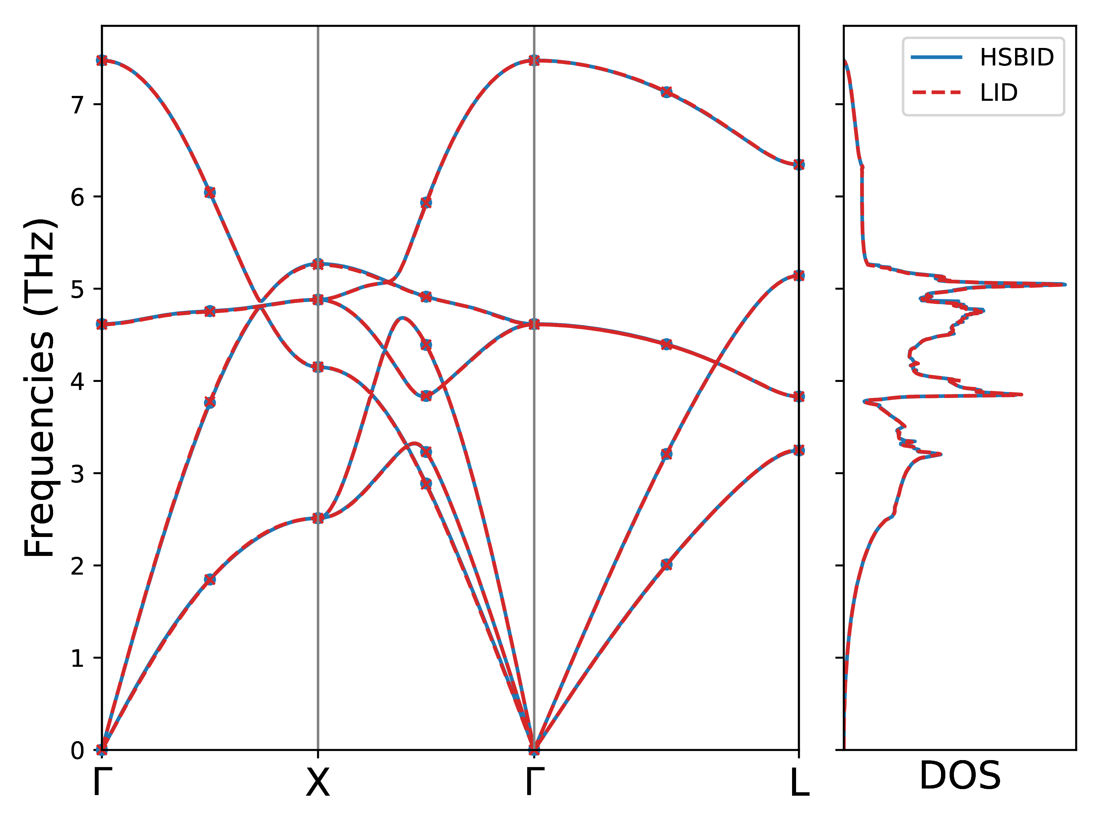
Fig. 12 Comparison between HS-BID and LID of Phonon and DOS of NaCl with FTG 4:math:hat{1} including LO-TO splitting, where the points are the phonons computed within the FTG and the lines are the Fourier interpolation from the FTG.
Phonon Linewidth and Thermal Conductivity
label{sec:si:phonon:linewidth}
With phonons and phonon interactions computed, we can use these coefficients to compute thermodynamic properties including phonon linewidth and thermal conductivity.
In this section, we will compute the phonon linewidth and thermal conductivity of \(\textrm{ThO}_2\) from its phonon interaction coefficients. For convenience of demonstration, we will interpolate the phonon interactions onto an FTG of \(3\hat{1}\) to integrate the \(\delta\)-functions to compute the linewidth and conductivity.
>>> pg = "Oh"
>>> supa = 3 * np.array([
      [1, 0, 0],
      [0, 1, 0],
      [0, 0, 1],
      ])
>>> temperature = np.linspace(0, 1000, 101)
>>> structure = get_structure(parse_poscar("tho2_linewidth/POSCAR"), stype=CrystalFTG)
>>> structure.species_names = ["Th", "O"]
>>> structure.orbitals = "p"
We can use the above configurations to construct the Conductivity object and assign the phonon interaction coefficients through the FourierInterpolation objects.
>>> cond = Conductivity(
        structure=structure,
        mesh=supa,
        pg=pg,
        )
>>> cond.set_Phi("tho2_linewidth/order2/fi_mesh444.hdf5",  order=2)
>>> cond.set_Phi("tho2_linewidth/order3/fi_meshsBcc.hdf5", order=3)
As an example, we can compute the phonon linewidth at \(\textbf{q} = \left(\frac{1}{2}, 0, 0\right)\) and the plot the different branches with respect to temperature the linewidth is evaluated at, shown in Fig. 13.
>>> qpoint = np.array(parse_array("1/2 0 0", dtype=Fraction))
>>> qpoint
array([Fraction(1, 2), Fraction(0, 1), Fraction(0, 1)], dtype=object)
>>> gamma = cond.gamma_tetra_at_phonon(qpoint=qpoint, temperature=temperature, phonon_cutoff=1.0E-4)
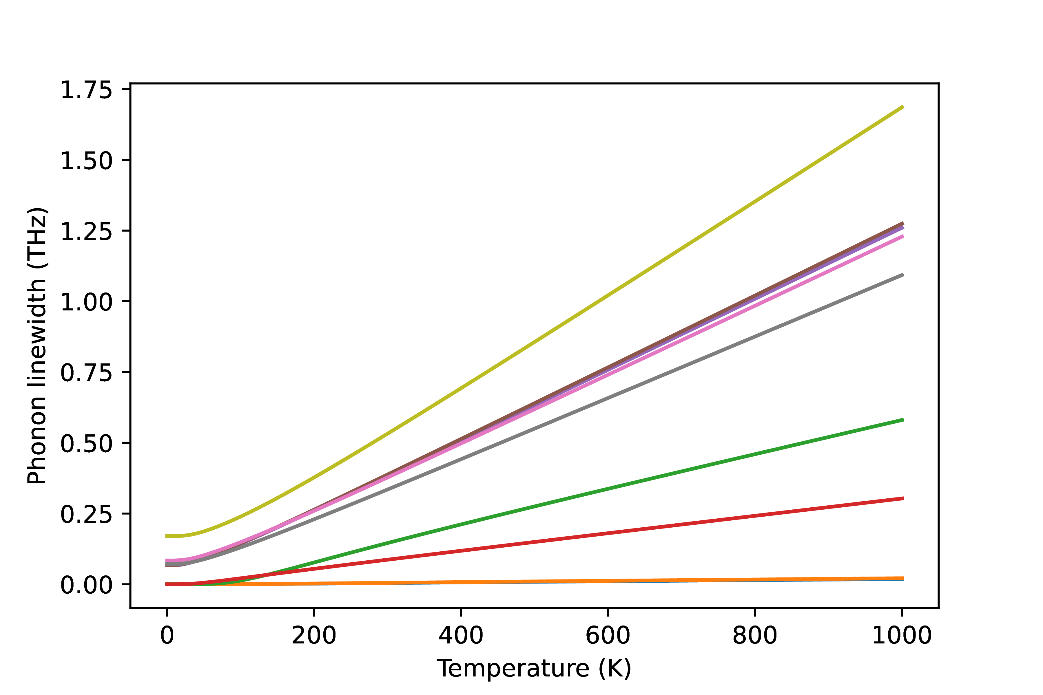
Fig. 13 Phonon linewidth of \(\textrm{ThO}_2\).
Additionally, we can also compute the thermal conductivity with relaxation time approximation, shown in Fig. 14.
>>> conductivity = cond.thermal_conductivity_RTA(temperature=temperature, phonon_cutoff=1.0E-4)
>>> x, y = np.array([(0, 0), (1, 1), (2, 2), (0, 1), (1, 2), (0, 2)]).T
>>> kappa = conductivity[:, x, y]
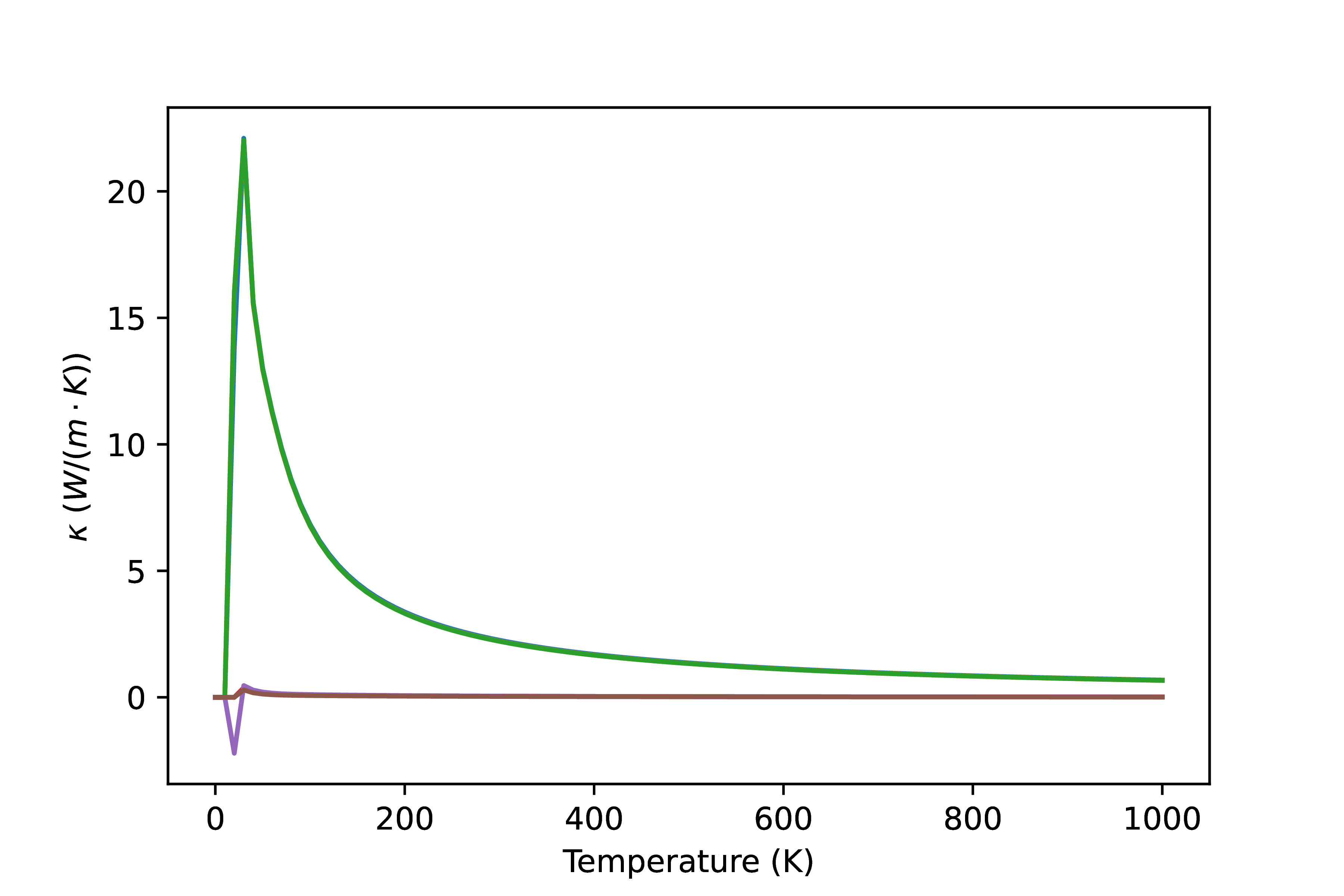
Fig. 14 Phonon conductivity of \(\textrm{ThO}_2\).