Strain Derivatives (strain_derivative)

Background and Basic Usage

Let us first unpack some data that we will need below.

# unpack data if not done yet
import numpy as np
import os
if not os.path.exists("data/nacl"):
  import tarfile
  tar = tarfile.open("data/nacl.tgz")
  tar.extractall(path='data/')
  tar.close()

Here we explore the strain_derivative class, which can be used to compute both linear and nonlinear elastic constants in crystals. This class does not do that much work: it mainly instantiates and uses several of our core classes. We begin with the generic considerations of how the class works. We will begin working with NaCl, given that it will be treated as an example below.

Let us begin by importing and instantiating the class. The constructor is listed for clarity.

def __init__(self,xtal,pgn,vname,order,target,fdtype='central',sim_trans=None,sim_trans_basis='standard',lattice_dim=3):

The variable xtal defines the crystal structure (a POSCAR for now). You will recognize familiar variable names from the finite_difference class. We will explore the variables "xx,yy" at order (1,1): a second derivative. Please note that you must specify a target, which is either energy or stress; and this is what you will be taking the derivative of.

At first, we will use the class in the simplest way possible: we will evaluate a specified energy derivative, without any considerations of group theory.

from strain_derivative import strain_derivative
sd=strain_derivative('data/nacl/c450_k20/static/POSCAR','Oh',['xx','yy'],[1,1],'energy')

The constructor will call the representation class which will symmetrize the strain tensor according to the provide point group: a variable called strain_rep will store this object.

print vars(sd.strain_rep).keys()
sd.strain_rep.irrep_counter

['dim', 'G', 'irrep_matr', 'chi', 'irrvec_dict', 'rank', 'rdim', 'pg', 'irrep_counter']

OrderedDict([('A1g', 1), ('Eg', 1), ('T2g', 1)])

The strain matrices are also stored in the ordereddict sd.strain_matr. We print them out here:

from IPython.display import display, Math,Markdown
from coordinate_tools import table_text as ttext
display(Math(r"\begin{align}"+"&&".join([r"\epsilon_{{{}}}=".format(s)+ttext(ss,cdelim='&',prec=None).latex().replace("0.5",r"\frac{1}{2}") for s,ss in sd.strain_matr.items()])+"\end{align}"))

$$\begin{align}\epsilon_{xx}=\begin{bmatrix} 1 & 0 & 0 \\ 0 & 0 & 0 \\ 0 & 0 & 0 \end{bmatrix}&&\epsilon_{yy}=\begin{bmatrix} 0 & 0 & 0 \\ 0 & 1 & 0 \\ 0 & 0 & 0 \end{bmatrix}&&\epsilon_{zz}=\begin{bmatrix} 0 & 0 & 0 \\ 0 & 0 & 0 \\ 0 & 0 & 1 \end{bmatrix}&&\epsilon_{xy}=\begin{bmatrix} 0 & \frac{1}{2} & 0 \\ \frac{1}{2} & 0 & 0 \\ 0 & 0 & 0 \end{bmatrix}&&\epsilon_{xz}=\begin{bmatrix} 0 & 0 & \frac{1}{2} \\ 0 & 0 & 0 \\ \frac{1}{2} & 0 & 0 \end{bmatrix}&&\epsilon_{yz}=\begin{bmatrix} 0 & 0 & 0 \\ 0 & 0 & \frac{1}{2} \\ 0 & \frac{1}{2} & 0 \end{bmatrix}\end{align}$$

You can review my course notes for more details on the above. Other important properties defined in the constructor are the standard basis (sbasis), irreducible basis (ibasis), and the transformed basis (tbasis):

print sd.sbasis
print sd.ibasis
print sd.tbasis

['xx', 'yy', 'zz', 'xy', 'xz', 'yz']
('A1g', 'Eg.0', 'Eg.1', 'T2g.0', 'T2g.1', 'T2g.2')
['v0', 'v1', 'v2', 'v3', 'v4', 'v5']

For multidimensional irreps, the row will always be denoted with a right period followed by an integer: Eg.0. If there are multiple instances of any irreps, these will be distinguished by a left period preceded by an integer: 1.A1g, etc. The transformed basis has been rotated by a matrix provided to the constructor, and this can be used to perform BID; but I will leave this for another part of the docs. For now we will either use the standard basis or the irreducible basis. The irreducible strain vectors can be seen in the standard variable of the representation instance (this class will be documented later).

print np.array(sd.strain_rep.irrvec)

[[ 0.57735027  0.57735027  0.57735027  0.          0.          0.        ]
 [ 0.70710678 -0.70710678  0.          0.          0.          0.        ]
 [-0.40824829 -0.40824829  0.81649658  0.          0.          0.        ]
 [ 0.          0.          0.          1.          0.          0.        ]
 [ 0.          0.          0.          0.          0.          1.        ]
 [ 0.          0.          0.          0.          1.          0.        ]]

There are a variety of methods which help you impart or measure strains, create directories, etc. However, I will only outline the higher level methods that bring everything together. In order to setup a calculation, the high level method to create all of the strain directories is:

def generate_fd_runs(self,delta,dname=None,dprefix='run',fpinp=None,zerodisp=False):

You must supply the delta, which has the same conventions as the finite_difference class, and everything else is optional. The variable dname provides a name for the overall directory that will hold the runs, and a default is chosen is nothing is provided; dprefix is the prefix for the subdirectories; fpinp is the location of the input files of the first-principles method which will be copied to every directory (e.g. INCAR, KPOINTS, etc if using VASP); zerodisp declares whether or not undistorted directories will be created.

The next major method is the one that collects all the data after the runs finish.

def gather_all_fp_data(self,fp_dirs,unstrained=None):

where fp_dirs is a list of first-principles directories that contain the data; and unstrained is a path to the unstrained data.

The next method simply instantiates the finite_difference class and feeds it the data.

def finite_difference(self,delta,use_available=False):

where these are standarad finite difference variables.

The next method instantiates the fit_quadratic class and feeds it the error tails.

def fit_quadratic(self,dmin=3,dmax=None,sigi=None,stype='consec'):

where these are standard fit_quadratic variables.

Finally, this method outputs the data to relevant files.

def output_data(self,sigi=None,units=None):

These are the basic methods that are called in the main program.

Examples

The above is best illustrated using a series of examples, and we will explore several:

1. Linear elastic constants of NaCl.
2. Linear and nonlinear elastic constants of ThO2.

NaCl

Let us start by creating the necassary directories.

%cd sample_mkruns

/home/cam1/git_projects/principia_materia_doc_v0/strain/sample_mkruns

We are starting in this directory with a directory containing the first-principles static calculation in a directory called static, which contains the static calculation of the undistorted structure, in addition to a yaml input file for strain_derivative.py.

%ls

inputs_mkruns.txt@  static@

!more inputs_mkruns.txt

delta: 0.005,0.03,0.005
fpinp: static/
order: 1
pgname: Oh
schema: mkruns
unstrained_path: static/
vname: A1g
xtal: static/POSCAR

Most of the variables should be clear.

fpinp - path to the input files for DFT. schema - mkruns tells us to generate the runs.

The above directory indicates that we will setup runs for the first derivative wrt to the A1g strain. However, please note that both first and second derivatives can be obtained from the same stencil. Now let us execute the code, and we can see all the runs that it has created. You will see that the highest level directory is called strain_A1g.

!strain_derivative.py -i inputs_mkruns.txt

%ls

inputs_mkruns.txt@  static@  strain_A1g/

%ls strain_A1g/

delta_0.5000/  delta_1.0000/  delta_1.5000/  delta_2.0000/  delta_2.5000/

%ls strain_A1g/delta_0.5000

run_m1/  run_p1/

%ls strain_A1g/delta_0.5000/run_m1

INCAR  info_strain.yaml  KPOINTS*  POSCAR  POTCAR

%ls strain_A1g/delta_0.5000/run_p1

INCAR  info_strain.yaml  KPOINTS*  POSCAR  POTCAR  WAVECAR@

Note how it has automatically created WAVECAR links in case you will run sequentially (XX add flag for this). Now let us clean up and look at some results. I have listed where you can find the runs in my dft_runs directory as well.

%rm -r strain_A1g

%cd ../data/nacl/c450_k20/

/home/cam1/git_projects/principia_materia_doc_v0/strain/data/nacl/c450_k20

%cat ../readme.txt # this is where the data was copied from

/home/cam1/dft_runs/nacl/pbe/c450_k20/

Here you can see that we have run a bunch of different strain derivatives. These are all either first or second derivatives. Please note that there is one cross derivative, denoted as strain_xx_yy.

%ls

inputs_energy_2.txt  static/       strain_T2g.0/  Untitled.png
inputs_mkruns.txt    strain_A1g/   strain_xx/
inputs_stress_1.txt  strain_Eg.0/  strain_xx_yy/

Here is our input file for processing these results.

%cat inputs_energy_2.txt

order: 2
pgname: Oh
target: energy
unstrained_path: static/
xtal: static/POSCAR
scale_delta: 0.5

Here we use the above input file and we add one more variable on the command line which tells us which data set to use. Please note that we have decided to take second order energy derivatives, and thus we must rescale the deltas using scale_delta by a factor of 0.5; because the grid was created for a first derivative, not a second derivative. Now let us run the code.

!strain_derivative.py -i inputs_energy_2.txt -dpath strain_A1g
!strain_derivative.py -i inputs_energy_2.txt -dpath strain_Eg.0
!strain_derivative.py -i inputs_energy_2.txt -dpath strain_T2g.0
!strain_derivative.py -i inputs_energy_2.txt -dpath strain_xx
!strain_derivative.py -i inputs_energy_2.txt -dpath strain_xx_yy -order 1,1 --scale_delta 1.

Here you can see the output file. The notiation -2 indicates that this is a second derivative. The first line is the output of our fit_quadratic function, and we are using default configurations, though you can pass configurations through argparse (see code).

!head -5 strain_A1g/Y_energy_A1g-2.txt

# 20.5300403857 340.287852585 0.00260950832044 [2, 3, 4]
#gy s=[0,o] l=[1,0] lw=2 lc=bu sfp=1 sfc=re sc=re ss=1.6 xr=0,0.012625 yr=20.26134,20.80196 sts=2 st=c\z{0.6}\v{-0.5}1\N=20.530
#gf 0,0.0125,-100,20.5300403857+340.287852585*x^2
0.00250000 20.59600000
0.00500000 20.46600000

We will want to compare our results to published results and experiment. Let us start with experiment.

Elastic constants of alkali halides at 4.2 degrees k
J. T. Lewis A. Lehoczky C. V. Briscoe
Physical Review 161 877 1967

They provide rather obscure units of \(10^{11}\) dyne/cm\(^2\), so we will use our units module to convert, and we will see a factor of 10 brings us to GPa.

from unit_conversion import pressure as units_pressure
1E11*units_pressure("dyne/cm^2","GPa")

10.0

Finally, we can see their results at T=4K in units of GPa (Table 4).

c\(_{11}\)	c\(_{12}\)	c\(_{44}\)
57.33	11.23	13.31

We can then rotate these results to the irreducible basis (see my class notes).

c\(_{A_{1g}}\)	c\(_{E_{g}}\)	c\(_{T_{2g}}\)
79.79	46.1	13.31

Perhaps it will be easiest to convert the above units into eV/(unit cell) by using the conversion between GPa and eV/A^3 and then multiplying by the volume. Let us do this.

from periodica import structure
xtal=structure('static/POSCAR')
conv=xtal.vol*units_pressure("GPa",'eV/A^3')
print "|".join(["{:.2f}".format(conv*s) for s in [79.79,46.1, 13.31]])
# 22.50|13.00|3.75
print "|".join(["{:.2f}".format(conv*s) for s in [57.33,11.23,13.31]])
# 16.17|3.17|3.75

So in units of eV/unit-cell, we have:

c\(_{11}\)	c\(_{12}\)	c\(_{44}\)
16.17	3.17	3.75

c\(_{A_{1g}}\)	c\(_{E_{g}}\)	c\(_{T_{2g}}\)
22.50	13.00	3.75

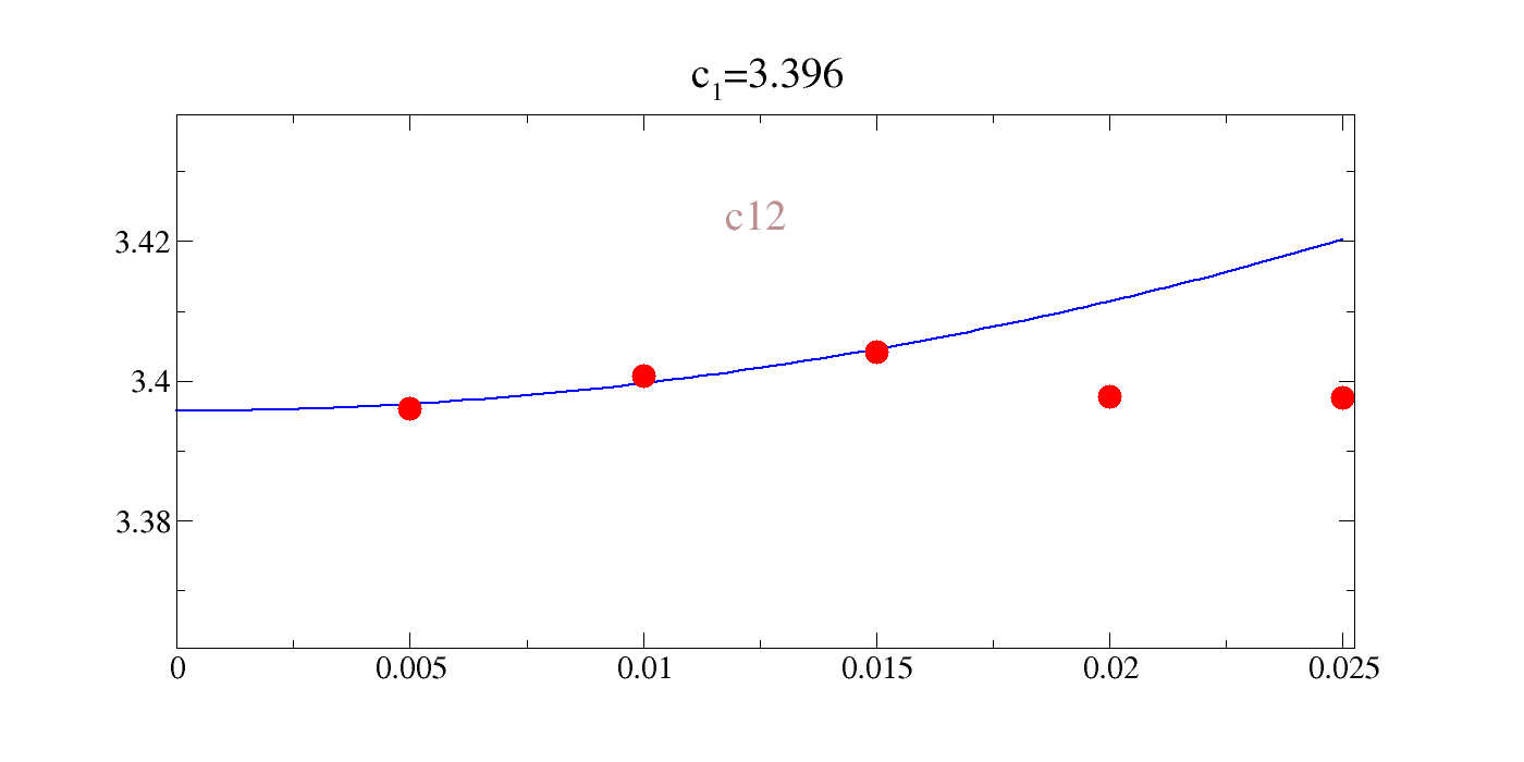
So now we know what the answers should roughly be. Let us first look at the irreducible measurements, then we can look at the direct measurement of \(c_{12}\).

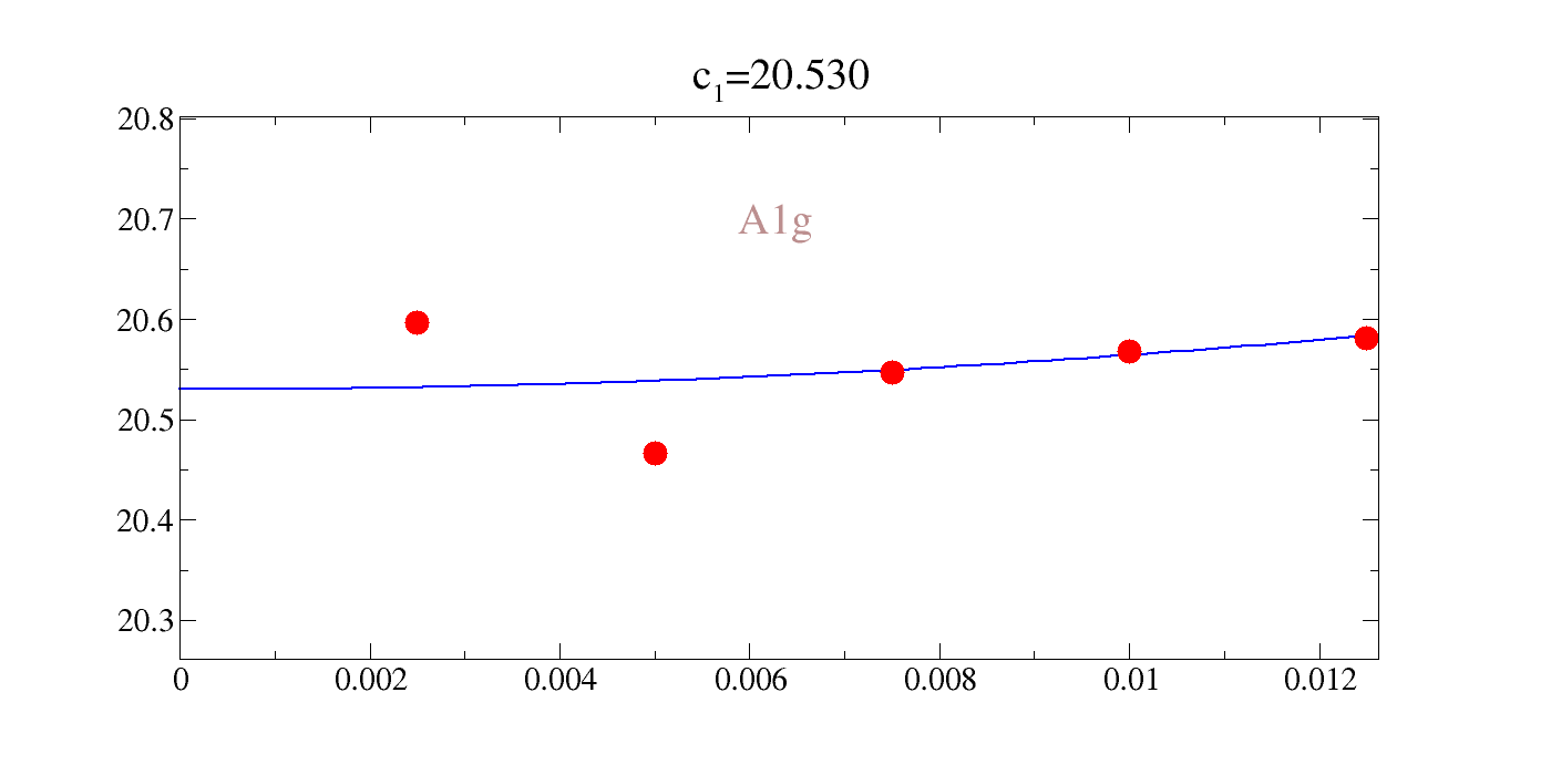
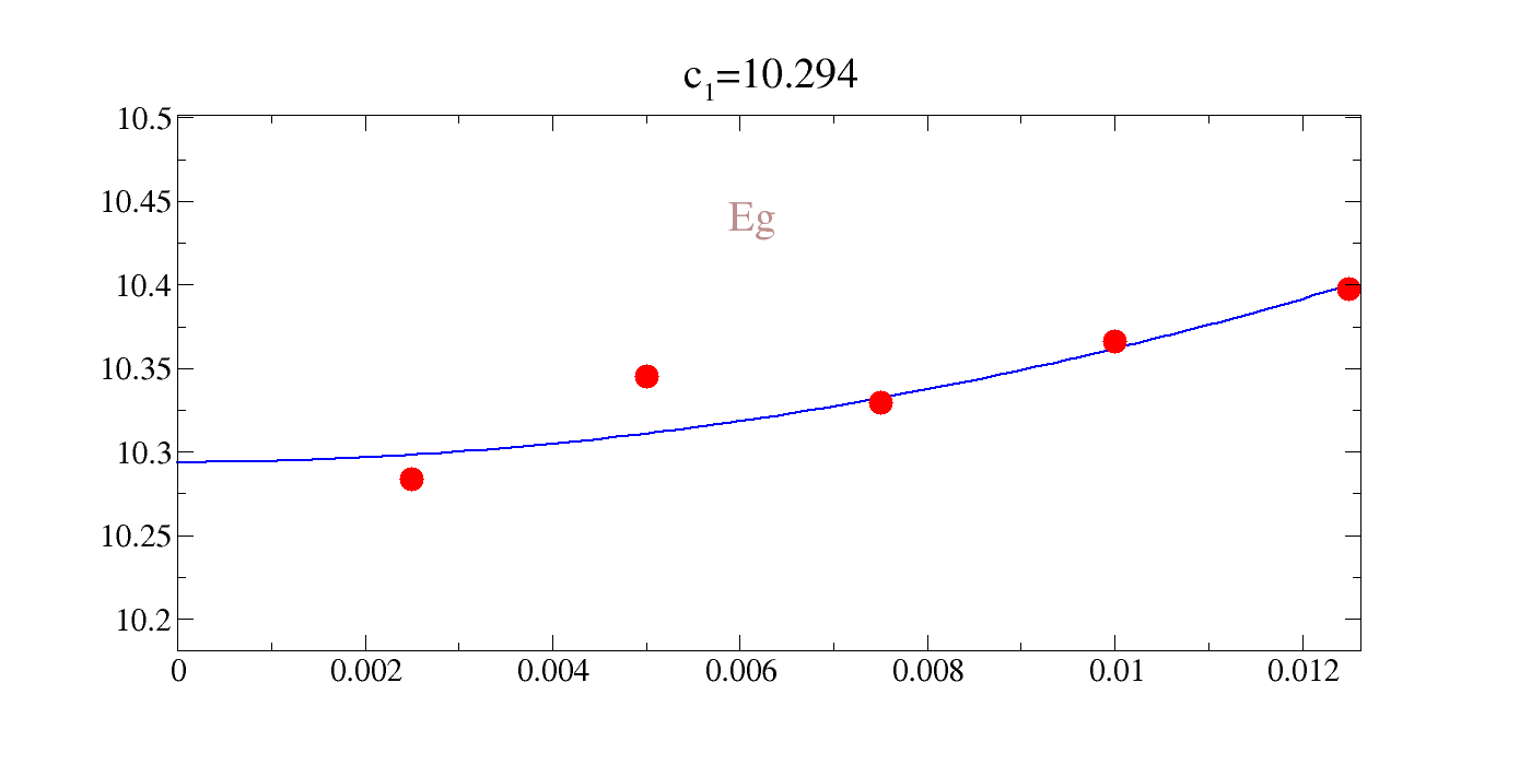
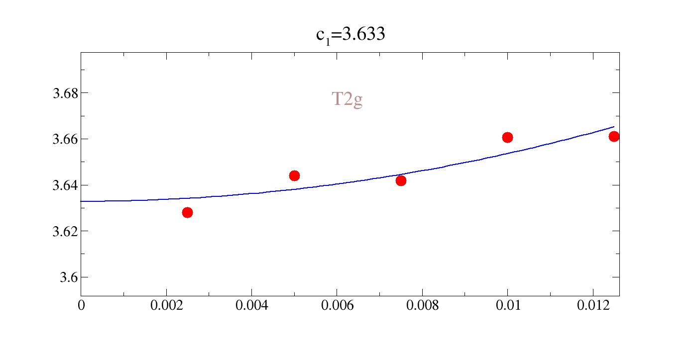
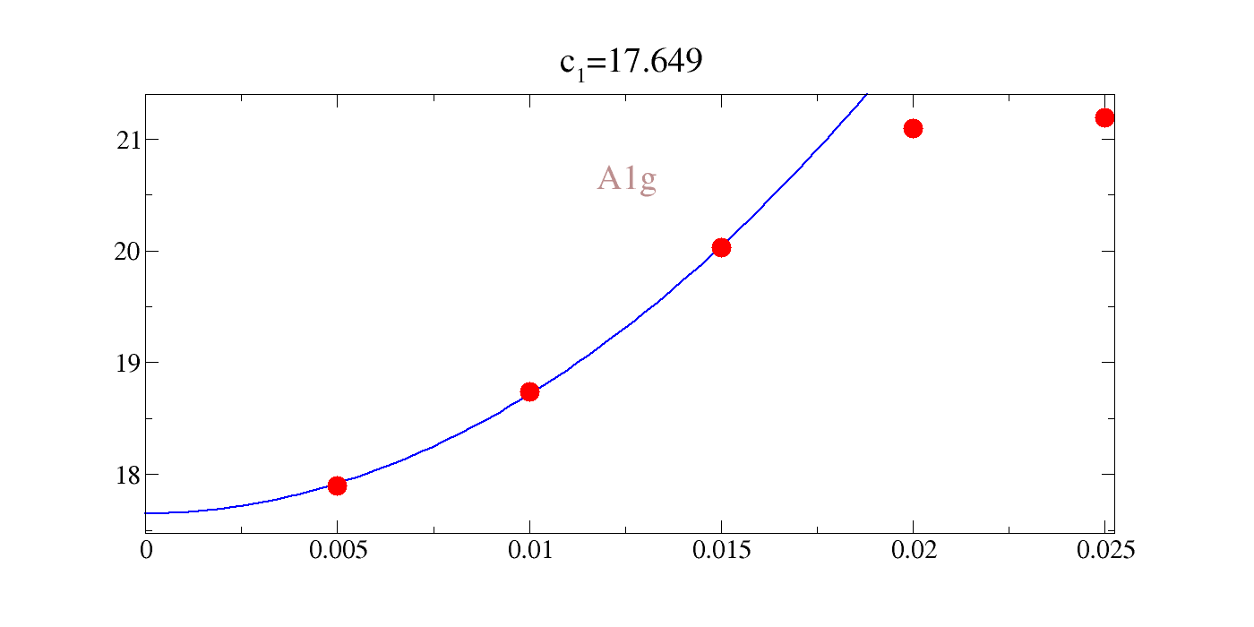
We could directly rangle the raw data, but the comments in the file are actually gracey commands such that we can easily interactively plot this. Our notation for the value of the intercept, inconveniently, is \(c_1\) in all cases; not to be confused with a given elastic constant. You can see that the agreement is pretty rough: 20-30%.

c\(_{A_{1g}}\)	c\(_{E_{g}}\)	c\(_{T_{2g}}\)
20.53	10.294	3.633

If we rerun things with LDA and the same parameters (not shown, but check my dft_runs directory):

c\(_{A_{1g}}\)	c\(_{E_{g}}\)	c\(_{T_{2g}}\)
25.26	15.12	3.39

Somewhat reassuringly, LDA and PBE bound the results in all cases except for the T2g modes (shear).

Let us look at all of the raw error tails.

!gracey.py -com strain_A1g/Y_energy_A1g-2.txt PNG strlt=view strc=br str=A1g,0.95,0.7
from IPython.display import Image
Image(filename='Untitled.png')

xmgrace -nosafe -noask -hardcopy -hdevice PNG -batch /home/cam1/.ppbatchfile

!gracey.py -com strain_Eg.0/Y_energy_Eg.0-2.txt PNG strlt=view strc=br str=Eg,0.95,0.7
Image(filename='Untitled.png')

xmgrace -nosafe -noask -hardcopy -hdevice PNG -batch /home/cam1/.ppbatchfile

!gracey.py -com strain_T2g.0/Y_energy_T2g.0-2.txt PNG strlt=view strc=br str=T2g,0.95,0.7
Image(filename='Untitled.png')

xmgrace -nosafe -noask -hardcopy -hdevice PNG -batch /home/cam1/.ppbatchfile

!gracey.py -com strain_xx_yy/Y_energy_xx_yy.txt PNG strlt=view strc=br str=c12,0.95,0.7
Image(filename='Untitled.png')

xmgrace -nosafe -noask -hardcopy -hdevice PNG -batch /home/cam1/.ppbatchfile

We do not need to use energy derivatives: we can also use stress. Let us take first derivatives of stress.

%cat inputs_stress_1.txt

pgname: Oh
target: stress
unstrained_path: static/
xtal: static/POSCAR
order: 1

On the command line, we add the variable sigi, which tells us which component of the stress to take the derivative wrt. Of course, you get all of them for free, and you can select whatever you want.

!strain_derivative.py -i inputs_stress_1.txt -dpath strain_A1g    -sigi A1g
!strain_derivative.py -i inputs_stress_1.txt -dpath strain_Eg.0   -sigi Eg.0
!strain_derivative.py -i inputs_stress_1.txt -dpath strain_T2g.0  -sigi T2g.0
!strain_derivative.py -i inputs_stress_1.txt -dpath strain_xx     -sigi xx
!strain_derivative.py -i inputs_stress_1.txt -dpath strain_xx     -sigi yy

Please note that this same stencil can also be used to obtain the second derivatives of stress.

!strain_derivative.py -i inputs_stress_1.txt -dpath strain_Eg.0  -sigi A1g -order 2 -scaled 0.5

Let us inspect one example, for the case of A1g. Here we see that the stress does not agree well with the energy. We would need to study the convergence parameters to see why (see my dft_runs directory). The example of ThO2 below shows nice agreement between energy and stress.

!gracey.py -com strain_A1g/Y_stress_A1g-2.txt PNG strlt=view strc=br str=A1g,0.95,0.7
Image(filename='Untitled.png')

xmgrace -nosafe -noask -hardcopy -hdevice PNG -batch /home/cam1/.ppbatchfile

ThO2

Linear Elastic (GGA)

%%capture
%cd ../..

Operationally, doing ThO2 is no different, so I will just provide the results (see my dft_runs directory for all the data). Units of GPa.

# /home/cam1/dft_runs/tho2/gga/c500_k20/irreducible_elastic
ls -d strain_{A1g,Eg.0,T2g.0}| robo_run.py 'pwd;head -2 Y_ener*2.txt|tail -1|pcol.py 3' fold=t | pcol.py 2|transpose.sh |format.sh 2
ls -d strain_{A1g,Eg.0,T2g.0}| robo_run.py 'pwd;head -2 Y_stre*2.txt|tail -1|pcol.py 3' fold=t | pcol.py 2|transpose.sh |format.sh 2

Target	c\(_{A_{1g}}\)	c\(_{E_{g}}\)	c\(_{T_{2g}}\)
Energy	572.51	246.68	79.43
Stress	570.25	244.79	78.29
Spunar	562.7	246.5	70.9

Here we see excellent agreement between energy and stress; and the published data of Spunar:

Theoretical investigation of structural and thermo-mechanical properties of thoria up to 3300 k temperature
B. Szpunar J. A. Szpunar
Solid State Sciences 36 35 2014

Nonlinear Elastic (GGA)

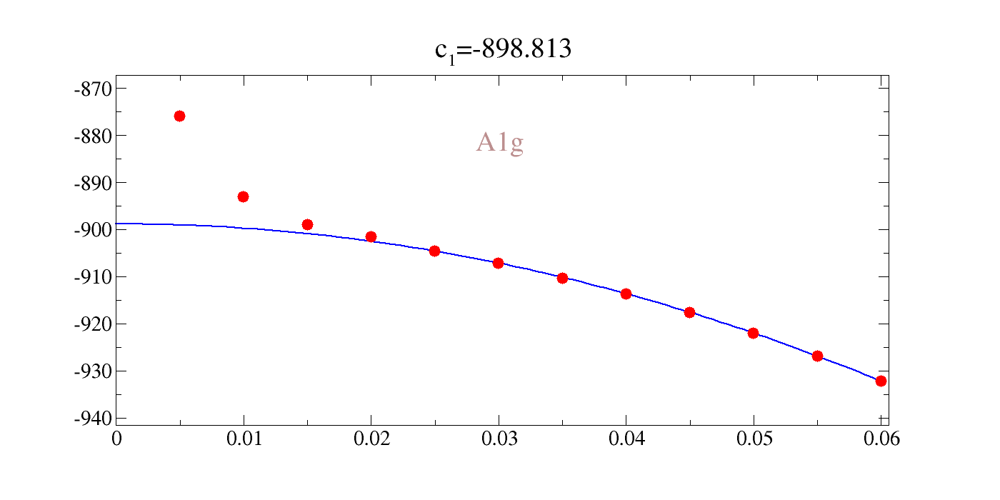
That is great, but we will also need the third and four derivatives of the energy with respect to the identity strain. Let us check out the results of the third derivative, for example:

!gracey.py -com tho2/Y_energy_A1g-3.txt PNG ss=1.2 strlt=view strc=br str=A1g,0.95,0.7
Image(filename='Untitled.png')

xmgrace -nosafe -noask -hardcopy -hdevice PNG -batch /home/cam1/.ppbatchfile

Let us tabulate some of these results.

\[ \Large \begin{align} \frac{\partial^2 E}{\partial \epsilon_{A_{1g}}^2}= 159 \,\,\textrm{eV/uc} && \hspace{4mm}&& \frac{\partial^3 E}{\partial \epsilon_{A_{1g}}^3}= -900 \,\,\textrm{eV/uc} && \hspace{4mm}&& \frac{\partial^4 E}{\partial \epsilon_{A_{1g}}^4}= 4258 \,\,\textrm{eV/uc} \end{align}\]

If we want to relate these to volumetric strain, we need to perform chain rule (see course notes on strain):

\[\Large \begin{align} \frac{d^3 E}{d \epsilon_{v}^3}&= \frac{d^3 E}{d \epsilon_{A_{1g}}^3} \left(\frac{d \epsilon_{A_{1g}}}{d \epsilon_{v}}\right)^3 + 3 \, \frac{d^2 E}{d \epsilon_{A_{1g}}^2} \frac{d \epsilon_{A_{1g}}}{d \epsilon_{v}} \frac{d^2 \epsilon_{A_{1g}}}{d \epsilon_{v}^2} \end{align}\]

where we have:

\[\Large \begin{align} \left.\frac{d \epsilon_{A_{1g}}}{ d\epsilon_{v} }\right|_{\epsilon_{v}=0} = \frac{1}{\sqrt3} && \left.\frac{d^2 \epsilon_{A_{1g}}}{ d\epsilon_{v}^2 }\right|_{\epsilon_{v}=0} =\frac{-2}{3\sqrt3} \end{align}\]

Plugging in, we see that:

\[\Large \frac{\partial^3 E}{\partial \epsilon_{v}^3}= -279 \,\,\textrm{eV/uc}\]

BID at second order (GGA)

It is useful to show how one can manually perform BID, measuring all the derivatives simultaneously. The runs can be found here.

/home/cam1/dft_runs/tho2/gga/c500_k20/bundled

There is a yaml input file called inputs_mkruns.txt with the following:

fpinp: ../static/
delta: 0.02,0.08,0.01
order: 1
pgname: Oh
schema: mkruns
unstrained_path: ../static/
vname: v0
xtal: ../static/POSCAR
_sim_trans:
  v0:
    A1g: 1.
    Eg.0: 1.
    T2g.0: 1.

You can see that we are taking the first derivative with respect to the variable v0, which is defined in the supplied similarity transformation sim_trans (the leading underscore means that it will bypass the parser). You can see that this new variable is equal parts A1g, Eg (zeroth row), and T2g (zeroth row). This will clearly probe all irreps, and because there are no repeating irreps, there is no interference. Therefore, we can measure all elastic constants via one stress derivative. Going into the following directory:

/home/cam1/dft_runs/tho2/gga/c500_k20/bundled/strain_v0

We can execute the following to extract all elements.

data_path: ./
pgname: Oh
target: stress
unstrained_path: ../../static/
xtal: ../../static/POSCAR
order: 1
units: GPa
sigi: A1g,Eg.0,T2g.0

We can add these results to our table.

Target	c\(_{A_{1g}}\)	c\(_{E_{g}}\)	c\(_{T_{2g}}\)
Energy	572.51	246.68	79.43
Stress (LID)	570.25	244.79	78.29
Stress (BID)	570.71	244.73	76.93
Spunar	562.7	246.5	70.9

Here you can see the advantage of BID: you get everything at sufficient precision from one measurement.

Linear and Nonlinear Elastic (LDA)

It is also interesting to explore more complicated derivatives. Let us consider the following two new ones, in addition to one previous one (but now with LDA, just because):

/home/cam1/dft_runs/tho2/lda/c500_k20/irreducible_elastic/strain_A1g-3
/home/cam1/dft_runs/tho2/lda/c500_k20/irreducible_elastic/strain_A1g_Eg.0-2
/home/cam1/dft_runs/tho2/lda/c500_k20/irreducible_elastic/strain_A1g_xx-2

\[\Large \begin{align} \hspace{-4mm} \frac{\partial^2 E}{\partial \epsilon_{A_{1g}}^2}= 170 \,\,\textrm{eV/uc} && \frac{\partial^2 E}{\partial \epsilon_{E_{g}^{(0)}}^2}= 67 \,\,\textrm{eV/uc} && \frac{\partial^2 E}{\partial \epsilon_{T_{2g}}^2}= 25.5 \,\,\textrm{eV/uc} && \frac{\partial^2 E}{\partial \epsilon_{xx}^2}= 101.4 \,\,\textrm{eV/uc} \end{align}\]

The latter derivative, with respect to \(\epsilon_{xx}\), can be obtained from the previous ones via the chain rule:

\[\begin{split}\Large \begin{align} \frac{\partial^2 E}{\partial \epsilon_{xx}^2}&= \frac{\partial^2 E}{\partial \epsilon_{A_{1g}}^2} \left( \frac{\partial \epsilon_{A_{1g}}}{\partial \epsilon_{xx}} \right)^2 + \frac{\partial^2 E}{\partial \epsilon_{E_{g}}^2} \left[ \left( \frac{\partial \epsilon_{E_{g}^{(0)}}}{\partial \epsilon_{xx}} \right)^2 +\left( \frac{\partial \epsilon_{E_{g}^{(1)}}}{\partial \epsilon_{xx}} \right)^2 \right] \\&= \frac{1}{3} \frac{\partial^2 E}{\partial \epsilon_{A_{1g}}^2} + \frac{2}{3} \frac{\partial^2 E}{\partial \epsilon_{E_{g}}^2} =101.3 \,\,\textrm{eV/uc} \end{align}\end{split}\]

We can see that it is nearly identical to the measured value.

Now for nonlinear.

\[\Large \begin{align} \hspace{-3mm} \frac{\partial^3 E}{\partial \epsilon_{A_{1g}}^3}= -957 \,\,\textrm{eV/uc} && \hspace{0mm} && \frac{\partial^3 E}{\partial \epsilon_{A_{1g}}\partial \epsilon_{E_{g}^{(0)}}^2}= -108 \,\,\textrm{eV/uc} && \hspace{0mm} && \frac{\partial^3 E}{\partial \epsilon_{A_{1g}}\partial \epsilon_{xx}^2}= -391 \,\,\textrm{eV/uc} \end{align}\]

Once again, we can obtain the latter derivative from the preceding two via the chain rule:

\[\Large \frac{\partial^3 E}{\partial \epsilon_{A_{1g}}\partial \epsilon_{xx}^2}= \frac{1}{3} \frac{\partial^3 E}{\partial \epsilon_{A_{1g}}^3} +\frac{2}{3}\frac{\partial^3 E}{\partial \epsilon_{A_{1g}}\partial \epsilon_{E_{g}^{(0)}}^2} = -391 \,\,\textrm{eV/uc}\]

The result obtained from the chain rule gives essentially identical results as compared to the direct measurement.

If we want to convert to volumetric strain, we have:

\[\Large \frac{\partial^3 E}{\partial \epsilon_{v}\partial \epsilon_{xx}^2}= \frac{1}{\sqrt3} \frac{\partial^3 E}{\partial \epsilon_{A_{1g}}\partial \epsilon_{xx}^2} =-226 \,\,\textrm{eV/uc}\]

The above result does not agree with what you would get if you manually computed the second derivative at a series of different volumes, given that such a procedure would change the reference of the strain. However, this is actually the quantity we want, because this is what is measured in experiment. In this case, you need to rebase the derivative. In other words, you need to renormalize strain such that it is measured from the expanded coordinate system (see course notes for derivation). We will denote the rebased strain as \(\mathcal{E}\). In this particular case, we have:

\[\Large \frac{\partial^3 E}{\partial \epsilon_{A_{1g}}\partial \mathcal{E}_{xx}^2} = \frac{\partial^3 E}{\partial \epsilon_{A_{1g}}\partial \epsilon_{xx}^2} + \frac{2}{\sqrt3} \frac{\partial^2 E}{\partial \epsilon_{xx}^2} = -273.9 \,\,\textrm{eV/uc}\]

Using the chain rule, we can then move to volumetric strain:

\[\Large \frac{\partial^3 E}{\partial \epsilon_{v}\partial \mathcal{E}_{xx}^2}= \frac{1}{\sqrt3} \frac{\partial^3 E}{\partial \epsilon_{A_{1g}}\partial \mathcal{E}_{xx}^2} = -158.1 \,\,\textrm{eV/uc}\]