Finite Difference (finite_difference)

General Background

Here we introduce the basic aspects of finite difference within the context of our PM code. Our class called finite_difference can be used to construct finite difference calculations for arbitrary numbers of variables, orders, and can be used for central, forward, or backward finite difference calculations. It will set up explicit grids for you to compute on, and it will also ensure that there are no redundant calculations due to overlapping deltas. If you collect and feed it the data, it will deliver the finite difference results.

Let us get started by importing the class:

import numpy as np
from general_finite_difference import finite_difference

The constructor only has one required parameter, which is called order. This variable order will be specified by a tuple of integers \(\large (n,m,\dots)\); where this means we are taking the n-th derivative of the first variable, m-th derivative of the second variable, etc. You can instead simply supply an integer \(\large n\), and this will imply that you are dealing with the n-th derivative of a function with respect to a single variable (though the function may depend on many variables). Let us envision working with a some potential energy \(\large V(x,y,z)\), or any function you like.

Single Variable

Let us begin by taking derivatives with respect to a single variable.

fd=finite_difference(2)

Given that we did not supply a variable name, via vname (tuple of strings), the code will name it using defaults.

fd.vname

['x']

Now let us look at one of the key dictionaries: stencil.

fd.stencil

OrderedDict([((-2,), 1), ((0,), -2), ((2,), 1)])

This corresponds to the usual formula for a single variable, and you can find something similar on the Wikipedia page, for example:

\[\Large V^{(n)}(2\Delta)=\frac{1}{(2\Delta)^n}\sum_{i = 0}^{n} (-1)^i \binom{n}{i} V\left(x + \left(n - 2i\right) \Delta\right)\]

Mathematically, you can see that our stencil dictionary stores the following information:

\[\Large\begin{aligned} \left((n - 2i,)\,\,,\,\,(-1)^i \binom{n}{i}\right) && \textrm{where} && i=1,..,n \end{aligned}\]

It is worth noting that we normally work with a rescaled function \(\large \tilde{V}^{(n)}(\Delta)=V^{(n)}(2\Delta)\), which is just a different convention. Both functions will have the the same intercept as \(\large\Delta\rightarrow0\), and will therefore deliver the same derivative. However, the quadratic error tail will be renormalized by a factor of 4, though we typically never exploit the error tail in any way: we just use it to ensure we are properly extrapolating to zero. We will not use the tilde notation in the future, but it will always be understood that our central finite difference uses this \(2\Delta\) convention; though this difference does not occur with forward or backward differences.

It might also be insightful to check out a 1st and 3rd derivative stencil.

fd1=finite_difference(1)
fd3=finite_difference(3)
print fd1.stencil
print fd3.stencil

OrderedDict([((-1,), -1), ((1,), 1)])
OrderedDict([((-3,), -1), ((-1,), 3), ((1,), -3), ((3,), 1)])

One of the nice parts of the code is that it can do forward and backward finite difference as well. The type of finite difference is specified on the constructor as fdtype, and has a default of central; though it can also take values of forward or backward.

fdf=finite_difference(2,fdtype='forward')
fdb=finite_difference(2,fdtype='backward')
print fdf.stencil
print fdb.stencil

OrderedDict([((0,), 1), ((1,), -2), ((2,), 1)])
OrderedDict([((-2,), 1), ((-1,), -2), ((0,), 1)])

Multiple Variables

Now let us move on to several variables: \(\large\frac{\partial^4V}{\partial x^2\partial y^2}\). In this case, we have order=(2,2):

fd=finite_difference((2,2))

Once again, the code will automatically supply names of the variables.

fd.vname

['x', 'y']

These names will suffice fine, but you can specify any names you like by supplying a list of names using the constructor variable name vnames. The only requirement for a name is that it must be a valid dictionary key. For example, if you are working with a function of strain, a rank two vector, you may prefer to choose different names:

fd=finite_difference((2,2),vname=['xx','yy'])
fd.vname

['xx', 'yy']

Now let us examine the stencil in this case.

fd.stencil

OrderedDict([((-2, -2), 1),
             ((-2, 0), -2),
             ((-2, 2), 1),
             ((0, -2), -2),
             ((0, 0), 4),
             ((0, 2), -2),
             ((2, -2), 1),
             ((2, 0), -2),
             ((2, 2), 1)])

Here, the code is simply evaluating the equation generalized to two variables with arbitrary order derivatives:

\[\Large V^{(n,m)}(2\Delta)=\frac{1}{(2\Delta)^{n+m}}\sum_{i = 0}^{n}\sum_{j = 0}^{m} (-1)^{i+j} \binom{n}{i}\binom{m}{j} V\left(x + \left(n - 2i\right) \Delta,x + \left(m - 2j\right) \Delta\right)\]

where the variable stencil is now storing:

\[\Large\begin{aligned} \left((n - 2i,m-2j)\,\,,\,\,(-1)^{i+j} \binom{n}{i}\binom{m}{j}\right) && \textrm{where} && i=1,..,n && j=1,..,m \end{aligned}\]

The code is general to arbitrary numbers of variables.

It is also useful to explore what stencil looks like in the case of forward finite difference. Here we only have positive displacements:

fd=finite_difference((2,2),fdtype='forward')
fd.stencil

OrderedDict([((0, 0), 1),
             ((0, 1), -2),
             ((0, 2), 1),
             ((1, 0), -2),
             ((1, 1), 4),
             ((1, 2), -2),
             ((2, 0), 1),
             ((2, 1), -2),
             ((2, 2), 1)])

Defining Deltas

Moving on, let us now actually define some \(\large\Delta\) to work with. Let us stick with a single variable and a second derivative:

fd=finite_difference((2,),delta=[0.01,0.02])

The first dictionary we create is the so-called delta_stencil. For a given value of delta, it tells which which stencil lattice points you need to evaluate. Furthermore, it knows when the stencil point are overlapping.

For this case below, the code knows not to add the 0 stencil point for a second time at the larger delta. This is a trivial case.

fd.delta_stencil

OrderedDict([(0.01, [(-2,), (0,), (2,)]), (0.02, [(-2,), (2,)])])

The next dictionary is delta_disp: for a given value of delta, it tells us what the actual displacement it. This is basically changing from stencil lattice coordinates to stencil cartesian coordinates.

fd.delta_disp

OrderedDict([(0.01, [(-0.02,), (0.0,), (0.02,)]), (0.02, [(-0.04,), (0.04,)])])

Finally, it might also be useful just to have a list of all displacements needed to be evaluated in order to perform FD, and this is stored in a list called all_disp.

fd.all_disp

[(-0.04,), (-0.02,), (0.0,), (0.02,), (0.04,)]

Now let us look at a slightly more interesting example with more deltas and a 4th order derivative. Here we see that the number of stencil points is cut in half every other delta due to the overlap.

fd=finite_difference((4,),delta=[0.01,0.02,0.03,0.04,0.05,0.06])

fd.delta_stencil

OrderedDict([(0.01, [(-4,), (-2,), (0,), (2,), (4,)]),
             (0.02, [(-4,), (4,)]),
             (0.03, [(-4,), (-2,), (2,), (4,)]),
             (0.04, [(-4,), (4,)]),
             (0.05, [(-4,), (-2,), (2,), (4,)]),
             (0.06, [(-4,), (4,)])])

Performing Finite Difference with Data

Our codes are set up to facilitate interacting with your data. One useful variable is all_disp_named, which includes the name of the variable along with the amplitude embedded in a table. This might be over the top, but I am paranoid of getting data mixed up.

fd=finite_difference((2,2),delta=[0.01])
fd.all_disp_named

[(('x', -0.02), ('y', -0.02)),
 (('x', -0.02), ('y', 0.0)),
 (('x', -0.02), ('y', 0.02)),
 (('x', 0.0), ('y', -0.02)),
 (('x', 0.0), ('y', 0.0)),
 (('x', 0.0), ('y', 0.02)),
 (('x', 0.02), ('y', -0.02)),
 (('x', 0.02), ('y', 0.0)),
 (('x', 0.02), ('y', 0.02))]

Given that your function will probably have more values that you are actively probing in a given derivative, you may want to take your above displacement and embed it in a larger number of variables; or change the order. Let us assume that you have a function of three variables x,y,z, then you can simply do:

fd.all_disp_fullarg("x y z".split())

[(-0.02, -0.02, 0.0),
 (-0.02, 0.0, 0.0),
 (-0.02, 0.02, 0.0),
 (0.0, -0.02, 0.0),
 (0.0, 0.0, 0.0),
 (0.0, 0.02, 0.0),
 (0.02, -0.02, 0.0),
 (0.02, 0.0, 0.0),
 (0.02, 0.02, 0.0)]

Now let us do some simple tests. Consider the following function:

\[\Large E(x)=\alpha_1x+\frac{1}{2}\alpha_2x^2+\frac{1}{6}\alpha_3x^3 +\frac{1}{24}\alpha_4x^4\]

where we have:

\[\Large \begin{align*} \alpha_1=2&&\alpha_2=3&&\alpha_3=5&&\alpha_4=160 \end{align*}\]

We will use the static method function_to_data, which takes a function as its argument, evaluates it over the grid, and then returns a dictionary of the data. This result is directly fed into the method eval_finite_difference, which actually puts everything together and performs the finite difference. This is the method that you will normally feed your first-principles data into.

alp1=2;alp2=3;alp3=20;alp4=160
def energy(x):
    return alp1*x+(1/2.)*alp2*x**2+(1/6.)*alp3*x**3+(1/24.)*alp4*x**4
results=fd.eval_finite_difference(fd.function_to_data(energy))
print results

OrderedDict([(0.01, 0.0)])

We will want to add a larger number of deltas so we have something interesting to look at. We do not have to reinstantiate the object in order to change the number of delta: we can simply call the method make_unique_disp; though there is nothing wrong with reinstantiating.

%%capture
fd.make_unique_disp(delta=np.arange(0.01,0.2,0.01))
results=fd.eval_finite_difference(fd.function_to_data(energy))

What would be even more interesting is to do a comparison between central and forward finite difference for this test function. Let us do it and then make a comparison plot.

delta=np.arange(0.01,0.2,0.01)
fdc=finite_difference((2,),delta=delta)
resultsc=fdc.eval_finite_difference(fdc.function_to_data(energy))
fdf=finite_difference((2,),delta=delta,fdtype='forward')
resultsf=fdf.eval_finite_difference(fdf.function_to_data(energy))

import matplotlib.pyplot as plt
plt.figure(figsize=(12,6))
plt.ylabel(r"$\frac{\partial^2E}{\partial x^2}$",**{'size':42,'rotation':0,'ha':'right'})
plt.xlabel(r"$\Delta$",**{'size':42})
plt.xticks(**{'size':22})
plt.yticks(**{'size':22})
plt.ylim([2.9,5.5])
plt.xlim([0,0.18])
plt.plot(*zip(*resultsc.items()),marker='o')
plt.plot(*zip(*resultsf.items()),marker='o')

[<matplotlib.lines.Line2D at 0x7f66f30a9090>]

Above you can see the major advantage of central finite difference: the error tail is quadratic instead of linear. The quadratic error tail is far more forgiving.

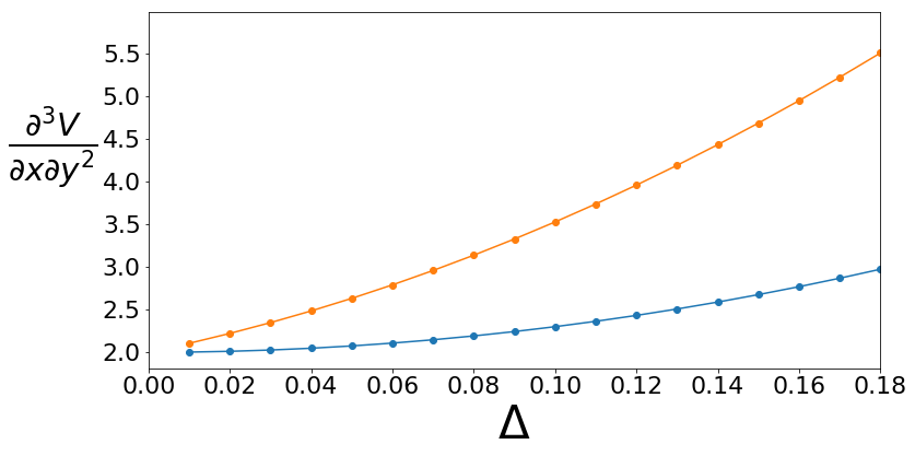
Now let us do a slightly more complicated function and a more complicated derivative. Consider the following function:

\[\Large V(x,y)=\alpha_1x+\frac{1}{2}\alpha_2x^2+\frac{1}{6}\alpha_3x^3 +\frac{1}{24}\alpha_4x^4+\alpha_5xy+\frac{1}{2}\alpha_6xy^2+\frac{1}{6}\alpha_7xy^3\]

where we have:

\[\Large \begin{align*} \alpha_1=2&&\alpha_2=3&&\alpha_3=5&&\alpha_4=160&&\alpha_5=1.5&&\alpha_6=2&& \hspace{4mm}\alpha_7=10 \end{align*}\]

def energy2d(x,y): return 5+2*x+0.5*3*x**2+(1/6.)*5*x**3+(1/24.)*160*x**4+1.5*x*y + 0.5*2*x*y**2+(1/6.)*10*x*y**3+(1/24.)*90*x*y**4

fdc2=finite_difference((1,2),delta=np.arange(0.01,0.2,0.01))
resultsc2=fdc2.eval_finite_difference(fdc2.function_to_data(energy2d))
fdf2=finite_difference((1,2),delta=np.arange(0.01,0.2,0.01),fdtype='forward')
resultsf2=fdf2.eval_finite_difference(fdf2.function_to_data(energy2d))

plt.figure(figsize=(12,6))
plt.ylabel(r"$\frac{\partial^3V}{\partial x\partial y^2}$",**{'size':42,'rotation':0,'ha':'right'})
plt.xlabel(r"$\Delta$",**{'size':42})
plt.xticks(**{'size':22})
plt.yticks(**{'size':22})
#plt.ylim([2.9,5.5])
plt.xlim([0,0.18])
plt.plot(*zip(*resultsc2.items()),marker='o')
plt.plot(*zip(*resultsf2.items()),marker='o')

[<matplotlib.lines.Line2D at 0x7f66f2f73110>]

Once again we see the benefits of central finite difference.

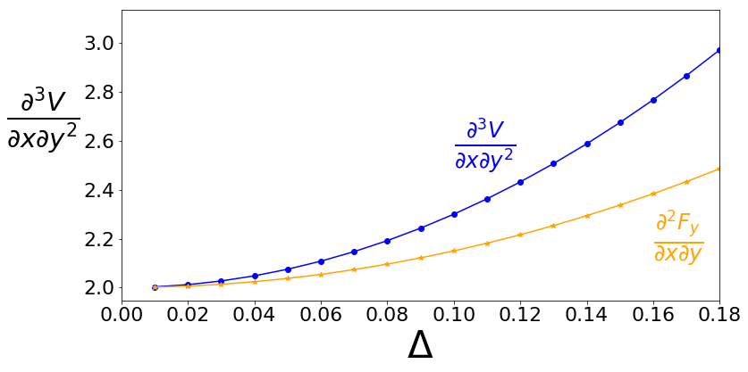
In order to make a connection with DFT, let us consider the possibility where we automatically have the first derivative using perturbation theory.

def forcex(x,y): return 3*x+(3/6.)*5*x**2+(4/24.)*160*x**3+1.5*y + 0.5*2*y**2+(1/6.)*10*y**3+(1/24.)*90*y**4
def forcey(x,y): return 1.5*x + 2*x*y+(3/6.)*10*x*y**2+(4/24.)*90*x*y**3
def force_vec(x,y): return (forcex(x,y),forcey(x,y))
fdc=finite_difference((1,1),delta=np.arange(0.01,0.2,0.01))
results=fdc.eval_finite_difference(fdc.function_to_data(force_vec))
results.items()[:3]

[(0.01, array([1.73472348e-14, 2.00150000e+00])),
 (0.02, array([0.   , 2.006])),
 (0.03, array([7.70988212e-15, 2.01350000e+00]))]

plt.figure(figsize=(12,6))
plt.ylabel(r"$\frac{\partial^3V}{\partial x\partial y^2}$",**{'size':42,'rotation':0,'ha':'right'})
plt.xlabel(r"$\Delta$",**{'size':42})
plt.xticks(**{'size':22})
plt.yticks(**{'size':22})
#plt.ylim([2.9,5.5])
plt.xlim([0,0.18])
plt.plot(*zip(*resultsc2.items()),marker='o',color='blue')
plt.plot(*zip(*[(s,ss[1]) for s,ss in results.items()]),marker='*',color='orange')
plt.text(0.16,2.15,r"$\frac{\partial^2F_y}{\partial x\partial y}$",fontsize=35,color='orange')
plt.text(0.1,2.55,r"$\frac{\partial^3V}{\partial x\partial y^2}$",fontsize=35,color='blue')

Text(0.1,2.55,'$\\frac{\\partial^3V}{\\partial x\\partial y^2}$')

We see that the two functions have the same intercept, but different values for the quadratic coefficient.