Extracting Error Tails (fit_quadratic)

Introduction

When using finite displacements, we are always faced with extrapolating to zero discretization. This class will help us fit either a pure quadratic or a pure linear function to data using different algorithms. At present, the fit_quadratic module is purely functional, not object oriented.

Our goal is to fit the coefficients \(c_1\) and \(c_2\) using least squares for a purely linear or purely quadratic function:

\[\Large \begin{align} f(x)=c_1+c_2x &&\hspace{5mm} f(x)=c_1+c_2x^2 \end{align}\]

We will need to have a function to perform linear least square (lls) under these conditions. The code to execute this task uses the psuedoinverse, and it is quite succinct.

def lls_quad(x,y,order=2):
  """Perform linear least squares for either a pure linear or pure quadratic function.
  """
  assert len(x)==len(y)
  dim=len(x)
  A=np.ones((dim,2),float)
  A[:,1]=poly(order)(x)
  c1,c2=np.dot(np.linalg.pinv(A),y)
  rmse=np.linalg.norm(c1+c2*poly(order)(x)-y)/np.sqrt(dim)
  return c1,c2,rmse

def poly(order):
  """Return either a linear or quadratic function.
  """
  assert (order==1 or order==2)
  return (lambda x:x**2) if order==2 else (lambda x:x)

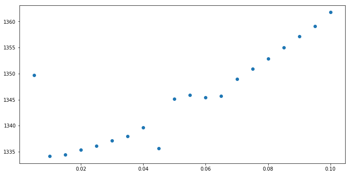
Let us use the data from Figure 4b of our paper to explore (PRB 100, 014303 (2019)).

from matplotlib import pyplot as plt
import numpy as np

data=np.loadtxt('data/example_tail.dat')
x,y=data[:,0],data[:,1]
plt.figure(figsize=(12,6))
plt.plot(x,y,'o')

[<matplotlib.lines.Line2D at 0x7fb0546dd0d0>]

Executing the code, we get the following:

import fit_quadratic as fit_quad
c1,c2,rmse=fit_quad.lls_quad(x,y)
print c1,c2,rmse

1336.3374703042705 2529.859880342763 3.505933707687217

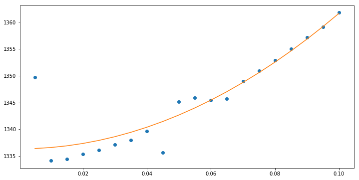
Above we see that the answer is given by the intercept \(c_1\). We also see that the root mean square error is rather small. Now let us plot the quadratic fit versus the data.

plt.figure(figsize=(12,6))
plt.plot(x,y,'o')
plt.plot(x,c1+c2*x**2)

[<matplotlib.lines.Line2D at 0x7fcde349f650>]

We can also perform a linear fit by changing order:

c1,c2,rmse=fit_quad.lls_quad(x,y,order=1)
plt.figure(figsize=(12,6))
plt.plot(x,y,'o')
plt.plot(x,c1+c2*x)

[<matplotlib.lines.Line2D at 0x7fcde3423d50>]

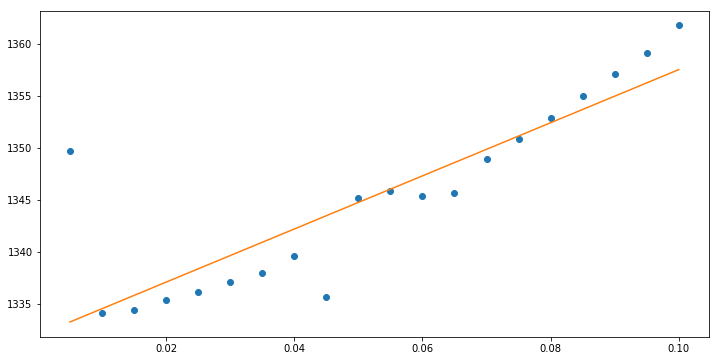
It is not always obvious what the optimal answer is. Nonetheless, the first point is clearly very far off and we do not want it included in the data to be fit. In general, we want some automated algorithm that will decide for us what data should be kept of thrown out. Basically, we want to explore the RMS error for different subsets of data and then pick the lowest one, subject to some relevant constraints.

Fitting over subsets of data

We need to provide a handful of functions in order to perform LLS on subsets of the provided data. First, consider the function min_over_subsets, which will perform LLS over some subsets of the data and find the minimum. Let us provide two subsets, and test this out.

fit_quad.min_over_subs(x,y,[[1,2,3,4],[2,3,4,5]])

(1333.6859441006618, 3975.5841461862437, 0.09985330879685789, [1, 2, 3, 4])

We see that it has the same output for as lls_quad, but now it also returns the subset that it used. When choosing subsets of a given size, two obvious choices come to mind. First, we could take all consecutive subsets of a given length. Second, we could take all combinations of a given length. This is accomplished using the make_subsets function, which takes the length of the data set, the length of the subset, and the type of subset.

print fit_quad.make_subs(8,3,stype='consec')
print
print fit_quad.make_subs(8,3,stype='combo')

[[0, 1, 2], [1, 2, 3], [2, 3, 4], [3, 4, 5], [4, 5, 6], [5, 6, 7]]

[(0, 1, 2), (0, 1, 3), (0, 1, 4), (0, 1, 5), (0, 1, 6), (0, 1, 7), (0, 2, 3), (0, 2, 4), (0, 2, 5), (0, 2, 6), (0, 2, 7), (0, 3, 4), (0, 3, 5), (0, 3, 6), (0, 3, 7), (0, 4, 5), (0, 4, 6), (0, 4, 7), (0, 5, 6), (0, 5, 7), (0, 6, 7), (1, 2, 3), (1, 2, 4), (1, 2, 5), (1, 2, 6), (1, 2, 7), (1, 3, 4), (1, 3, 5), (1, 3, 6), (1, 3, 7), (1, 4, 5), (1, 4, 6), (1, 4, 7), (1, 5, 6), (1, 5, 7), (1, 6, 7), (2, 3, 4), (2, 3, 5), (2, 3, 6), (2, 3, 7), (2, 4, 5), (2, 4, 6), (2, 4, 7), (2, 5, 6), (2, 5, 7), (2, 6, 7), (3, 4, 5), (3, 4, 6), (3, 4, 7), (3, 5, 6), (3, 5, 7), (3, 6, 7), (4, 5, 6), (4, 5, 7), (4, 6, 7), (5, 6, 7)]

Clearly, consecutive creates many fewer subset. We can now use these in min_over_subsets; let us explore subsets of length 4. Rather than having to enter this function manually, we provide a wrapper for min_over_subs which indicates that the min is being performed at constant subset type and size (ts).

print fit_quad.min_over_subs_at_ts(x,y,4,stype='consec')
print fit_quad.min_over_subs_at_ts(x,y,4,stype='combo')

(1336.2001081303704, 2607.4008334790706, 0.02900291530967237, [13, 14, 15, 16])
(1334.6874234166858, 2709.2952389247075, 0.010673836206792539, [5, 6, 18, 19])

We see that the subset of length 4 with minimum RMSE cannot be reached using the consecutive subsets.

Now, we may want to compare subset of different lengths, so we have a function that will loop over a range of subset sizes for a fixed subset type. Given that smaller subsets will normally have smaller error, we need to somehow penalize smaller subsets.

ac1,ac2,armse,asub=fit_quad.min_over_subs_at_t(x,y,smin=4,smax=None,stype='consec',penalty=lambda x:1./x)
bc1,bc2,brmse,bsub=fit_quad.min_over_subs_at_t(x,y,smin=4,smax=6,   stype='combo', penalty=lambda x:1./x)
print ac1,ac2,armse,asub
print bc1,bc2,brmse,bsub

1336.2001081303704 2607.4008334790706 0.02900291530967237 [13, 14, 15, 16]
1334.6874234166858 2709.2952389247075 0.010673836206792539 [5, 6, 18, 19]

We see that subsets of length 4 are selected in both cases. We could make the penalty function more severe if we want to push the solution to larger subset sizes; but we leave this for now. Let us look at the results.

plt.figure(figsize=(12,6))
plt.plot(x,y,'o',color='blue')
plt.plot(x,ac1+ac2*x**2,color='red')
plt.plot(x,bc1+bc2*x**2,color='green')
plt.plot(x[asub],y[asub],'o',color='red')
plt.plot(x[bsub],y[bsub],'o',color='green')

[<matplotlib.lines.Line2D at 0x7fce10a12710>]

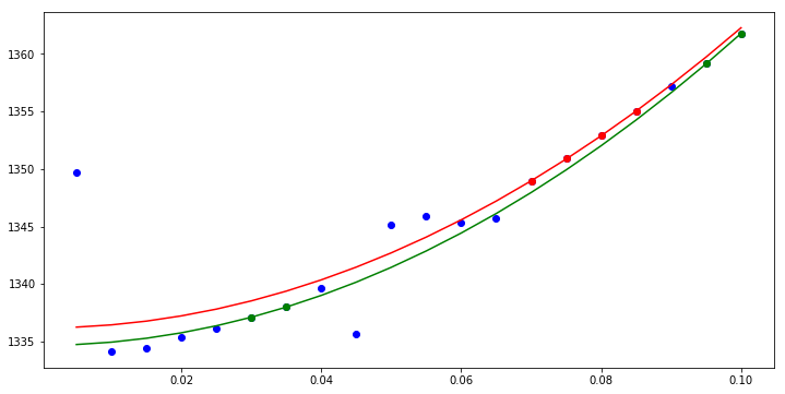
Here we have colored the points to indicate which points were selected in each respective fit: blue were not used, red were consec, and green were combo.

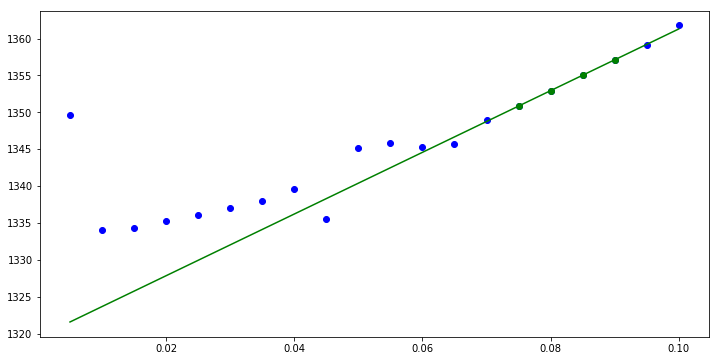
If we were doing forward finite difference, we would want to fit to a linear curve, not a quadratic. Fortunately, all of this machinery is general to that case, and we simply need to supply order=1. Let us do an example:

c1,c2,rmse,sub=fit_quad.min_over_subs_at_ts(x,y,4,stype='consec',order=1)
plt.figure(figsize=(12,6))
plt.plot(x,y,'o',color='blue')
plt.plot(x,c1+c2*x,color='green')
plt.plot(x[sub],y[sub],'o',color='green')

[<matplotlib.lines.Line2D at 0x7fcde3289b10>]

Using code from command line

We will want to be able to use this code from the command line when exploring, and we can. Our inputs will be as follows:

parser.add_argument('-order',help='Either fit pure linear (1) or pure quadratic (2).',default=2,type=int)
parser.add_argument('-stype','--subset_type', help='Type of subsets which may be automatically chosen.',choices=['consec','combo'],default='consec')
parser.add_argument('-ssize','--subset_size', help='Size of subset to explore.',default=None,type=int)
parser.add_argument('-smin', help='Minimum subset size to search over.',default=None,type=int)
parser.add_argument('-smax', help='Maximum subset size to search over.',default=None,type=int)
parser.add_argument('-sub',help='Perform lls on given subset.', type=lambda s: [int(tt) for tt in s.split(',')] )
parser.add_argument('file', help='Name of the input file.')
parser.add_argument('-p','--plot', help='Plot the data along with the resulting fit.',action='store_true')

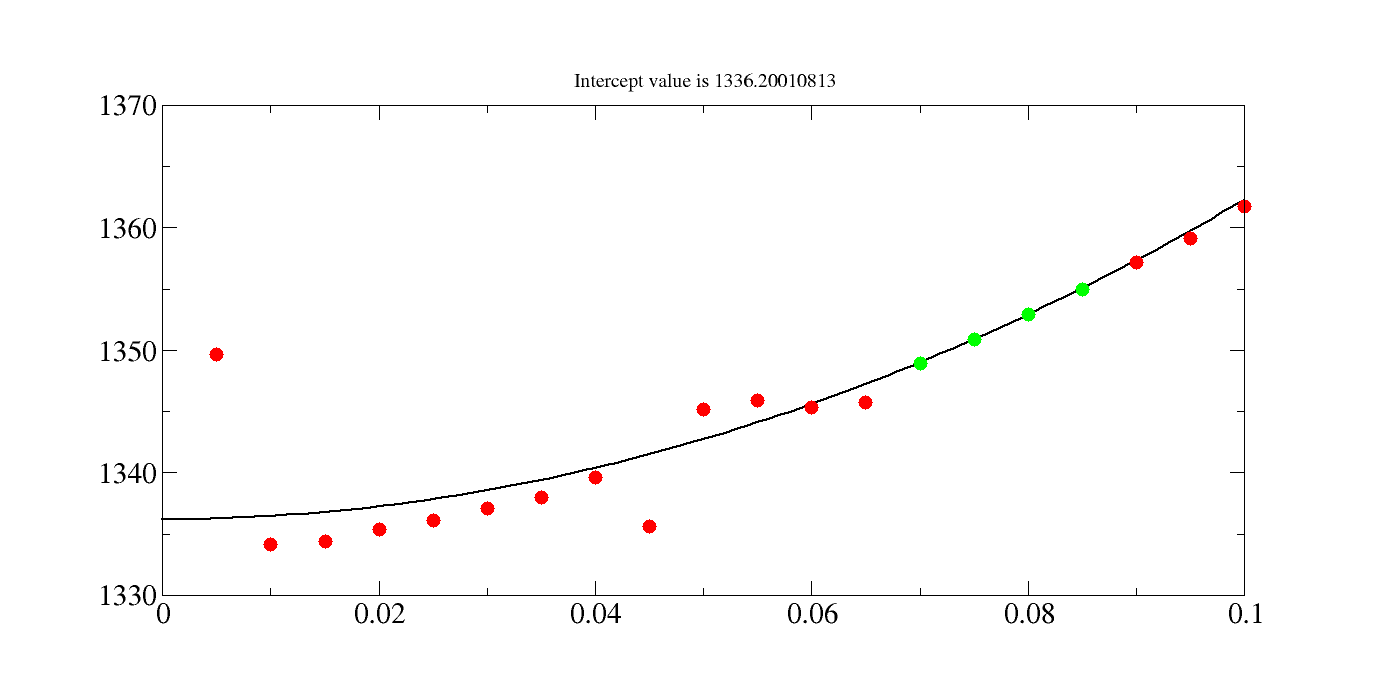
Here is a typical example from the command line.

!fit_quadratic.py data/example_tail.dat -ssize 4 -stype consec

c0  c1  RMSE  subset
1336.20010813 2607.40083348 0.0290029153097 [13, 14, 15, 16]

If you have xmgrace installed, you can also interactively see a plot using -p (or get a png with -pp).

!fit_quadratic.py data/example_tail.dat -ssize 4 -stype consec -pp
from IPython.display import Image
Image(filename='Untitled.png')

c0  c1  RMSE  subset
1336.20010813 2607.40083348 0.0290029153097 [13, 14, 15, 16]
xmgrace -nosafe -noask -hardcopy -hdevice PNG -batch /home/cam1/.ppbatchfile