VASP SrVO3 Band structures
INPUT: INCAR | KPOINTS | POTCAR | POSCAR | kinput
OUTPUT: OSZICAR | OUTCAR | EIGENVAL
Here we compute the band structure using VASP. A band structure plot normally consists of plotting the Kohn-Sham eigenvalues as a function of the reciprical lattice vector for some arbitrarlily chosen path through k-space. Typically one will enumerate all of the high-symmetry points and then take paths connecting them. You must decide what path you would like to take through k-space. Of course, one cannot do a self-consistent calculation with an arbitrary k-point set. Therefore, one must first do a calculation to obtain the converged density, and then one can do a non-self-consistent calculation at an arbitrary set of k-points using the previously converged density. In VASP terminology, we will do the following:
Perform a static self-consistent calculation as usual.
Make a new directory and start with your four usual input files in addition to the CHGCAR file from the previous step. Several flags must be added to the input:
ICHARG=11
ISMEAR=0
The ISMEAR parameter does not have to be zero, but it cannot be -5 because that will give an error, and a nonintuitive one at that! Additionally, you must manually creat a KPOINTS file. I have an old script that does this. We will create an input file called kinput:
$ cat kinput

0.0 0.0 0.0  G
0.5 0.0 0.0  X
0.5 0.5 0.0  M
0.5 0.5 0.5  R
0.0 0.0 0.0  G

$ kgenerator.pl 20   # The number indicates how many points between each high symmetry point.

$ head -5 kpoints
auto generate
81
Reciprocal
0.0 0.0 0.0 1
0.025 0 0 1

$ mv kpoints KPOINTS
You will see that the run will converge quickly as the charge density is fixed. The eigenvalues are stored in a file called EIGENVAL. We will show the first few lines of it here:
   5    5    1    1                                                          # Not useful
 0.1148420E+02  0.3857953E-09  0.3857953E-09  0.3857953E-09  0.5000000E-15   # Not useful
 1.000000000000000E-004                                                      # Not useful
 CAR                                                                         # Not useful
unknown system                                                               # INCAR title
  33   81   20                                                               # ? N_kpts N_bands

 0.0000000E+00  0.0000000E+00  0.0000000E+00  0.1234568E-01   # kx ky kz weight (fractional coordinates)
  1      -29.5334                                             # band1
  2      -14.4218                                             # band2
  3      -13.2295                                             # band3
  etc ...
 20        6.0336                                             # band20

 0.2500000E-01  0.0000000E+00  0.0000000E+00  0.1234568E-01   # kx ky kz weight
  1      -29.5332                                             # band1
  2      -14.4220                                             # band2
  etc ...
Please note that if the system were spin polarized then there would be two real numbers listed for each band (ie. up and down). So now we have the raw eigenvalues listed at each k-point. We will also need to know the fermi energy, but this must be determined from the static calculation. Let us assume that it is one directory up in a directory called static, then you would extract it as follows:
$ grep E-fermi ../static/OUTCAR
 E-fermi :   4.9664     XC(G=0): -11.4721     alpha+bet :-13.1640
Now we would like to plot the eigenvalues. There is a nice script to do this, though it has not been fully documented yet. We will just use it for now:
bands_plot.py outfile=bands.out fermi=../static/OUTCAR
# bands.out will be like:
# kdist1  band1 band2 ... band20
# kdist2  band1 band2 ... band20
# etc
The bands_plot script will do something additional that is nice, which is to create a set of comments at the beginning of the file that will draw vertical lines at the high symmetry points in addition to creating labels which were given in the kinput file (if given). One can then plot this using gracey or whatever they like:
gracey.py -com bands.out
Below I have copied the comment lines out of bands.out and used them to make a gracey plot from within python.
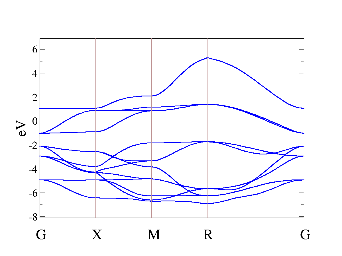
Bands. This is the band structure for SrVO3.
EPS
Plotting Script