VASP Fat Band structures for Graphene on Cu

INPUT: INCAR | KPOINTS | POTCAR.gz | POSCAR | kinput

OUTPUT: PROCAR.gz | OUTCAR_static.gz

Here we make a fat band plot. First, follow the regular procedure for performing a band structure. The only difference is that you must add LORBIT=11 to the INCAR. We can then run fat_bands_vasp.py to extract the bands and the projections from the PROCAR; it will look in the OUTCAR of a static run for the Fermi energy (speficied on command line). This program outputs three columns (kdist, band energy, projection), and a space will be printed before it moves on the next band. The file will be quite long given that this printout happens for every single band. The option “con” simply tells the program how to format the projection (ie. add/multiply something or not). If “fat” is given, then you get the raw projection out of the PROCAR.

On the command line, we need to specify: atom1 atom2 orbital1 orbital2 [OUTCAR] [con=fat]. This will sum the projection over the range from atom1-atom2 and orbital1-orbital2. This code is very primitive and needs to be rewritten, but for now it does the job.

fat_bands_vasp.py 4 5 pz pz staticrun/OUTCAR con=fat > bands_pz.out

Now that we have the output, let us plot it using gracey.py. We read in the file, scale the projection in a way we like, and then make the contour plot. This can be done using the size of a point (ie. fat_contour) or by the color of the point (ie. contour method, not shown).

# now read in the fat bands file and rescale the third column to a sensible point size...
# i have rescaled to a number betwen 0 and 1... and then taken the sqrt and multiplied by
# a constant. You may want to tweak this part to your liking...
INP=open("bands_pz.out",'r')
OUT=open('/tmp/bands1.out','w')
for ii in INP:
    if ii.split():
      if ii.strip()[0]!='#':
        l=[float(s) for s in ii.split()]
        # this is an error function scaling if you like...
        #nv=l[2]*20
        #nv=0.5*(erf(nv*5-2.5)+1)*0.6
        #OUT.write("%s %s %s\n"%(l[0],l[1],nv))
        # power scaling...
        OUT.write("%s %s %s\n"%(l[0],l[1],l[2]**0.8*1.02))
    else: OUT.write("\n")
OUT.close()

aa=plot()
aa.fat_contour("/tmp/bands1.out")
# most of this is autogenerated from running "plotbands.py plines=t"
aa.quickin(r"""
lines=3 linel=0,0,3.958796,0 xa=off lines=1 linec=bl
ymin=-10 ymax=4 yt=2 xmin=0 xmax=3.95879552497
linel=1.448439,ymin,1.448439,ymax
linel=2.284512,ymin,2.284512,ymax
str=\v{-0.8}\h{-0.25}\xG,0.020000,ymin-0.1
str=\v{-0.8}\h{-0.25}M,1.408439,ymin-0.1
str=\v{-0.8}\h{-0.25}K,2.284512,ymin-0.1
str=\v{-0.8}\h{-0.25}\xG,3.958796,ymin-0.1
pr=800,600 lc=bu yl=eV s=o sfp=1 sfc=re sc=re  lw=1.2
""")

aa.picname='fat_band_plot_cu'
aa.show()
aa.show('EPS')

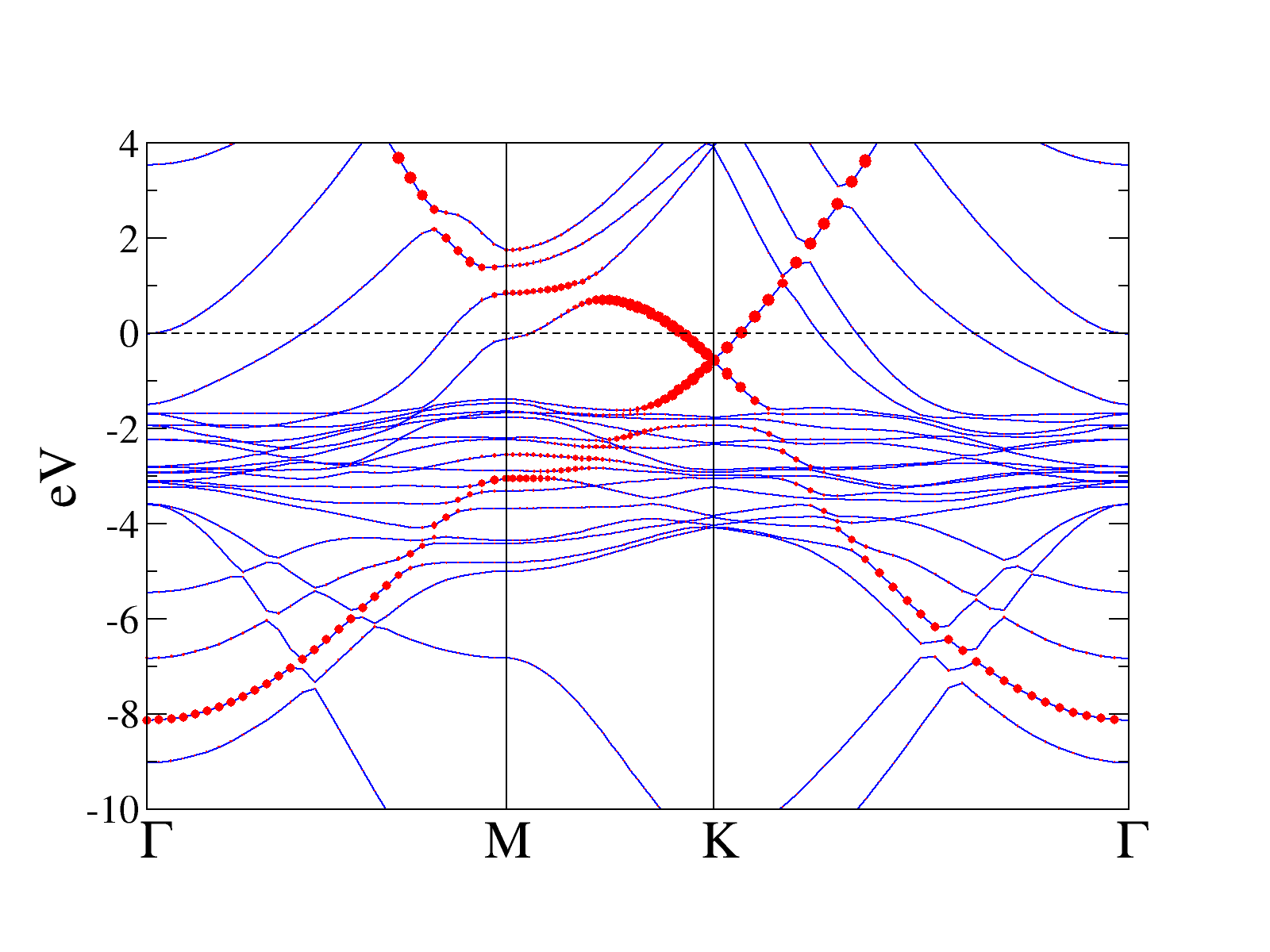
Bands. This is the band structure for graphene sitting on top of Cu. PDF