Linear Response U¶

Introduction¶

Here I (Eric) discuss computing Hubbard U via the linear response approach in VASP. You should first read M. Cococcioni and S. de Gironcoli, Phys. Rev. B 71, 035105 (2005) to understand the theory. The basic idea is that we are applying a potential to the correlated (I’ll refer to them as d states in this document) levels of a single site and observing how this changes the d occupancies on all the sites. This tells us about the screened on-site Coulomb interaction.

In principal we need to perform three types of calculations:

normal DFT calculation ( $\alpha=0$ )
charge-self-consistent calculations for a series of finite $\alpha$ (“interacting” response)
non-charge-self-consistent calculations for a series of finite $\alpha$ (“bare” response)

The first type gives us the number of d electrons ( $N_d$ ) and the charge density for the unperturbed ( $\alpha=0$ ) system. For the second and third types we read in this charge density via the CHGCAR file (which also includes the density matrices) and apply a finite $\alpha$ . In the second type we allow the charge density to relax to help screen this perturbation, while for the third type we do not.

I typically use $\alpha$ values of $\pm$ 0.08, $\pm$ 0.05, and $\pm$ 0.02, which in my experience usually falls within the linear regime of $N_d$ vs. $\alpha$ .

1-shot versus 2-shot approaches¶

Note that in the Cococcioni paper (and in Quantum ESPRESSO) people typically look after the first electronic iteraction (i.e., before the charge density is updated for the first time) to obtain the bare response. We call this the “1-shot” approach. In principle this is a fine thing to do provided one uses exact diagonalization or sufficiently converges the iterative diagonalization before updating the charge density for the first time (e.g. by making NELMDL more negative). However, empirically we find that this approach DOES NOT work in VASP and underestimates U by approximately 1 eV. After extensive testing, our best understanding is that VASP is doing something strange for the charge-self-consistent run that is enabling more screening of $\alpha$ than should be present after the first electronic step if the charge density were really not yet changed. Therefore, one should do separate calculations to obtain the bare and interacting responses, which we call the “2-shot” approach.

What VASP executable should I use?¶

vasp.5.3_wei¶

We have a modified version of VASP (vasp.5.3_wei) written by Wei Xie in Dane Morgan’s group that implements the potential perturbation $\alpha$ . One can successfully compute U using this code, but there is some extra work involved. For bare (non-charge-self-consistent) runs the density matrix printed out by VASP is just that read in from the CHGCAR file initially and does not reflect the effects of the finite $\alpha$ . If we were just doing something like computing a DFT+U band structure, this would be a reasonable thing for VASP to do since we know the potential based on that density and density matrices is already correct. However, in our case this is problematic since $\alpha$ is actually changing the density matrices in some way about which we care.

Therefore, one needs to play a trick of saving the WAVECAR from the bare run, reading it into a 1-electronic-step (NELM=1) charge-self-consistent run to compute and print the actual density matrices corresponding to the WAVECAR. This takes some extra time and requires more (temporary) hard disk storage, so it is undesirable. However, the approach does work so let me know if you want to use it and I can explain how to use the executable.

LDAUTYPE=3 in VASP 5¶

We discovered computing linear response U with the 2-shot approach is actually a hidden feature in VASP 5 using the LDAUTYPE=3 tag. The only information on this is on this VASP forum post. This post includes instructions on how to run the calculations. Basically you need to set LDAUTYPE=3 as well as the LDAUU and LDAUJ parameters, which are now used as the $\alpha$ parameters for the up and down spin channels, respectively, instead of the U and J values. For computing U one should apply the potential to both spin channels so the parameters LDAUU and LDAUJ should be identical.

One subtlety is that for this method the site at which the perturbation is applied must be listed as its own atomic species. So the POSCAR and POTCAR need to be modified to reflect this. For example, for iron (Fe) if we are using an 8-atom unit cell we should split this up into 1 species with 1 ion and 1 species with 7 ions and include the Fe pseudopotential twice in POTCAR. LDAUU and LDAUJ should have finite value only for this first atomic species since we only want to apply the perturbation to a single site as opposed to all of them.

Another very important subtetly we have found empirically is a difference in sign convention for the LDAUTYPE=3 method. Basically we believe the $\alpha$ applied is actually $-\alpha$ , so you should flip the signs of all your $\alpha$ . This will restore the expected behavior that negative $\alpha$ should lead to increased $N_d$ on this site of the perturbation.

For LDAUTYPE=3 calculations the density matrices themselves are not printed but one can just find the trace (which is all we need) from bottom of the OUTCAR file (making sure LORBIT=11 so this is computed).

Calculating U¶

One can perform linear regression on the $N_d$ vs. $\alpha$ data to get the elements of the first row of the response matrices $\chi$ (when using data from the interacting runs) and $\chi_0$ (when using data from the bare runs). To fill in the rest of the upper right half of each matrix, one can use the symmetry of the lattice since each site in the supercell is related to the perturbed site via a translation vector of the primitive unit cell. Finally, one can fill in the bottom left half of the matrices trivially since these matrices are symmetrics again due to the symmetry of the lattice.

At the end of the day, one looks at the first diagonal entry of $\chi_0^{-1}-\chi^{-1}$ to get U (in the same units as $\alpha$ , which are eV).

Important: One needs to keep increasing the size of the supercell for these calculations until the value of U stops changing.

resp_mat.f90¶

There is a code called resp_mat.f90 written by Cococcioni that you can find by searching around Quantum ESPRESSO tutorials for LDA+U. This code will do the postprocessing computation described in the previous section. It also has implemented the option to explicit enforce charge neutrality (see his paper) to speed up convergence with respect to supercell. In addition, it has implemented the extrapolation to larger supercell also discussed in that paper. I have found this code to be useful to check my own results. Documentation is in the comments of the source code, but let me know if you have any questions. One word of caution: at some point I think I saw a post in the Quantum ESPRESSO forum suggesting there might be a bug in this code for hexagonal unit cells.

Some example data¶

Here is some example data for ferromagnetic Fe for a 2x2x2 supercell of the primitive bcc unit cell using the 2-shot approach.

Note: For this case I am not enforcing charge neutrality or extrapolating to larger unit cell.

POSCAR KPOINTS POTCAR

$\alpha=0$ INCAR:

LWAVE = .FALSE.
LCHARG = .TRUE.
NELM = 50
ISYM = 0
ISPIN = 2
LMAXMIX = 4
LASPH = .TRUE.
LORBIT = 11
EDIFF = 1E-6
ISMEAR = -5
PREC = Accurate
ENCUT = 500.000
NEDOS = 2000
MAGMOM = 1*2 7*2
LDAU = .TRUE.
LDAUTYPE = 3
LDAUPRINT = 2
LDAUU = 0.0 0
LDAUJ = 0.0 0
LDAUL = 2 -1

$\alpha=0.05$ bare INCAR:

ICHARG = 11
LWAVE = .FALSE.
LCHARG = .FALSE.
NELM = 50
ISYM = 0
ISPIN = 2
LMAXMIX = 4
LASPH = .TRUE.
LORBIT = 11
EDIFF = 1E-6
ISMEAR = -5
PREC = Accurate
ENCUT = 500.000
NEDOS = 2000
MAGMOM = 1*2 7*2
LDAU = .TRUE.
LDAUTYPE = 3
LDAUPRINT = 2
LDAUU = -0.05 0
LDAUJ = -0.05 0
LDAUL = 2 -1

$\alpha=0.05$ interacting INCAR:

ISTART = 0
ICHARG = 1
LWAVE = .FALSE.
LCHARG = .FALSE.
NELM = 50
ISYM = 0
ISPIN = 2
LMAXMIX = 4
LASPH = .TRUE.
LORBIT = 11
EDIFF = 1E-6
ISMEAR = -5
PREC = Accurate
ENCUT = 500.000
NEDOS = 2000
MAGMOM = 1*2 7*2
LDAU = .TRUE.
LDAUTYPE = 3
LDAUPRINT = 2
LDAUU = -0.05 0
LDAUJ = -0.05 0
LDAUL = 2 -1

Note that LDAUU and LDAUJ use -0.05 instead of 0.05 due to the different sign convention mentioned above.

Here I plot $N_d$ vs $\alpha$ for each of the 8 Fe ions in the supercell. Solid (dashed) lines correspond to the bare (interacting) response. The line colors correspond to different Fe ion indices.

../../_images/n_vs_alpha.png — $N_d$ vs. $\alpha$ (`EPS`)¶

First of all you can see that the magnitude of the changes of $N_d$ is much larger for the bare case than the interacting case, which makes sense since for the former the charge density is unable to screen the perturbation. Secondly, you can notice that for the on-site response (that of ion 1, the site at which $\alpha$ is applied, in blue) $N_d$ increases for negative $\alpha$ , which makes sense since lowering the potential encourages more electrons to occupy the orbitals on that site. Finally, you can observe that the response for both the bare and the interacting cases are largest for ion 1 and decay away from this site. You might notice that in this system the interacting response is very small for all the ions other than the first, which might be explained by the fact that we have a metallic system so the screening is very efficient.

$\chi_0$

-1.2075	0.1554	0.1430	0.1312	0.1419	0.1253	0.1403	0.1581
0.1554	-1.2075	0.1312	0.1430	0.1253	0.1419	0.1581	0.1403
0.1430	0.1312	-1.2075	0.1554	0.1403	0.1581	0.1419	0.1253
0.1312	0.1430	0.1554	-1.2075	0.1581	0.1403	0.1253	0.1419
0.1419	0.1253	0.1403	0.1581	-1.2075	0.1554	0.1430	0.1312
0.1253	0.1419	0.1581	0.1403	0.1554	-1.2075	0.1312	0.1430
0.1403	0.1581	0.1419	0.1253	0.1430	0.1312	-1.2075	0.1554
0.1581	0.1403	0.1253	0.1419	0.1312	0.1430	0.1554	-1.2075

$\chi$

-0.2054	0.0075	0.0032	0.0108	0.0086	0.0048	0.0070	0.0113
0.0075	-0.2054	0.0108	0.0032	0.0048	0.0086	0.0113	0.0070
0.0032	0.0108	-0.2054	0.0075	0.0070	0.0113	0.0086	0.0048
0.0108	0.0032	0.0075	-0.2054	0.0113	0.0070	0.0048	0.0086
0.0086	0.0048	0.0070	0.0113	-0.2054	0.0075	0.0032	0.0108
0.0048	0.0086	0.0113	0.0070	0.0075	-0.2054	0.0108	0.0032
0.0070	0.0113	0.0086	0.0048	0.0032	0.0108	-0.2054	0.0075
0.0113	0.0070	0.0048	0.0086	0.0108	0.0032	0.0075	-0.2054

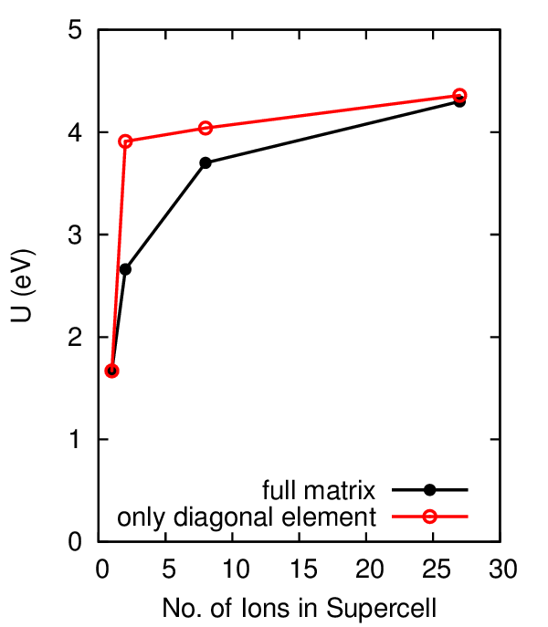
Here is a plot of the computed U in eV versus the size of the supercell. You can see that U increases with supercell size and starts to saturate a bit above 4 eV. The results from the full matrix inversion are shown in black, while the results one obtains from only using the diagonal elements of $\chi$ and $\chi_0$ are shown in red.

../../_images/u_vs_supa.png — Computed U vs. supercell size (`EPS`)¶