Special Quasi-random Structures (SQS)

Basic Idea

Here I (Eric) discuss generating special quasirandom structures (SQS) using the Alloy Theoretic Automated Toolkit (ATAT). You should first read S.-H. Wei et al., Phys. Rev. B 42, 9622 (1990) and A. Zunger et al., Phys. Rev. Lett. 65, 353 (1990) to understand the theory. The basic idea is to generate a minimally-sized supercell that approximates a random (disordered) solid solution. This could be an alloy or a system with disordered vacancies, for example. The goal, which was formulated in the context of the cluster expansion, is to find a supercell whose cluster correlation functions as best as possible match those of the random structure.

Tutorial

There are generally four parts of this method:

0. creation of proper input files

1. calculation of target correlations of random structure

2. generation of structures of particular size based on such target correlations

3. evaluation of candidate structures based on correlations with heightened number of clusters

Below I discuss each step and include data for an example of Li_0.5CoO₂. I am assuming you have successfully compiled ATAT on your machine (which was as simple as typing “make” if I recall).

Step 0: Create Input Files

One needs a lattice file (lat.in) containing the crystal structure of the primitive unit cell and a structure file (conc.in) that is used to determine the composition. The papers A. van de Walle et al., Calphad 26, 539 (2002) and A. van de Walle, Calphad 33, 266 (2009) as well as this ATAT manual page discuss the format of these files.

Li_0.5CoO₂ example: lat.in conc.in

This is a relaxed non-spin-polarized PBE structure of LiCoO₂. Notice that in Li and Vac are listed at the 0.5,0.5,0.5 site in lat.in to indicate that the alloy is of Li and vacancies on this sublattice. The structure in conc.in is irrelevant except for the fact that it indicates we are interested in .

Step 1: Calculation of Target Correlations

corrdump -noe -2=3 -3=3 -4=0 -rnd -l=lat.in -s=conc.in > tcorr.out

The corrdump code calculations cluster correlations. “noe” indicates that we ignore the empty cluster. The “l” and “s” flags specify the lattice and structure files, respectively. The “rnd” flag indicates we want the correlations of the random structure (since our target is to mimic these correlations).

The number flags specify cutoffs (in ) for what clusters are considered (2 for pair, 3 for triplet, 4 for quadruplet, etc.). If a cluster (collection of point sites) contains any intersite distance greater than the flag value (cutoff), then the cluster is not included. For example, since we have “-3=3” we only have triplets with intersite distances less than 3 . In this case the in-plane 1st nearest neighbor (nn) is 2.85 and the next nearest intersite distance is greater than 3 so we only include triplets with a maximum intersite distance corresponding to the in-plane 1st nn. To see a picture of this distance in the structure, you can look at Figure 7 of A. Van der Ven et al., Phys. Rev. B 58, 2975 (1998).

Step 2: Generation of Structures

The gensqs code (see documentation) generates SQS structures. The clusters and target correlations files generated by the previous step are indicated by the “cf” and “tc” flags, respectively. The “n” flag dictates the size of the supercell desired and represents the total number of atoms and vacancies. In this example I am looking for Li₆Co₁₂O₂₄.

gensqs -n 48 -cf=clusters.out -tc=tcorr.out > sqs.out

Note that the computation increases rapidly as a function of n. If you need very large supercells, you might be interested in checking out a Monte Carlo algorithm for this process as described in A. van de Walle et al., Calphad 42, 13 (2013) and this documentation page.

Step 3: Evaulation of Structures

The sqs.out file will contain SQS structures that meet the target correlations. If there are none, one can use more lax target correlations (fewer clusters).

Presumably there will be several or many candidate structures. Now one must evaluate which is the best. To do so, we consider more clusters by increasing our max intersite distance cutoffs. For example, here we choose 8.6 for pairs, triplets, and quadruplets taking us out to a maximum intersite distance corresponding to the inter-plane 6th nn.

Note that we must always compare correlations of a candidate structure to those of the random structure corresponding to the same clusters. So we use corrdump to compute the correlations of the candidate structures as well as the random alloy.

corrdump -noe -2=8.6 -3=8.6 -4=8.6 -l=lat.in -s=sqs.out > tcorr_final.out

corrdump -noe -2=8.6 -3=8.6 -4=8.6 -l=lat.in -s=sqs.out -rnd > tcorr_finalRND.out

Finally for each structure one can calculate a figure of merit (fom), the square root of the sums of the squares of the correlation function differences [candidate (in tcorr_final.out) compared to random (in tcorr_finalRND.out)]. In these files each column corresponds to a cluster. The smaller the fom the better. This is like taking the RMS of the cluster correlations but without dividing by the number of clusters since I think this quantity makes more sense if it’s extensive with the number of clusters (though this will not change the structure you choose in the end).

One should keep increasing the number of clusters until it is clear which one or few candidate SQS structures are the best. In addition, to gain more confidence in the answer one should also repeat the procedure with different initial target correlations.

Finally, one can see how the fom (at the same level of clusters) changes as one increases the supercell size. Of course, increasing the supercell size adds more degrees of freedom to emulate a random structure so the fom should decrease.

SQS Images (EPS)

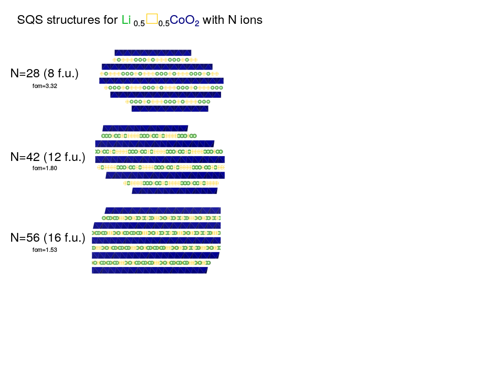
You can see a significant drop in the fom between N=28 and N=42 and then a smaller decrease going from N=42 to N=56.

Another useful tutorial: SQS Tutorial