One-Band Hubbard Model

This tutorial focuses on the one-band Hubbard model.

Cubic lattice

Let us start by going over a simple example where we can anticipate the answers. First let us consider the Hubbard model on the cubic lattice. First, we need to supply the structure and what type of orbitals we are using. We adopt a similar file to the POSCAR in VASP:

Hubbard model
1
1 0 0
0 1 0
0 0 1
1
d
0 0 0   s

We also need to give the real space Hamiltonian as a python dictionary. This should be stored in a file:

t=1/6.
Hopping={}
Hopping[( 1, 0, 0)]=[[t]]
Hopping[(-1, 0, 0)]=[[t]]
Hopping[( 0, 1, 0)]=[[t]]
Hopping[( 0,-1, 0)]=[[t]]
Hopping[( 0, 0, 1)]=[[t]]
Hopping[( 0, 0,-1)]=[[t]]

Assuming that the structure is put into a file called “poscar” and the Hamiltonian is put in a file called “rham.py”, we would run the following command to compute the DOS:

$ tb_tools.py dens=1.0 ham=rham.py nk=20 pos=poscar tdos=t pg=oh

One is also free to put the commands in a file (I usually use inputs.inp) and then call the program as follows:

$ tb_tools.py -i inputs.inp

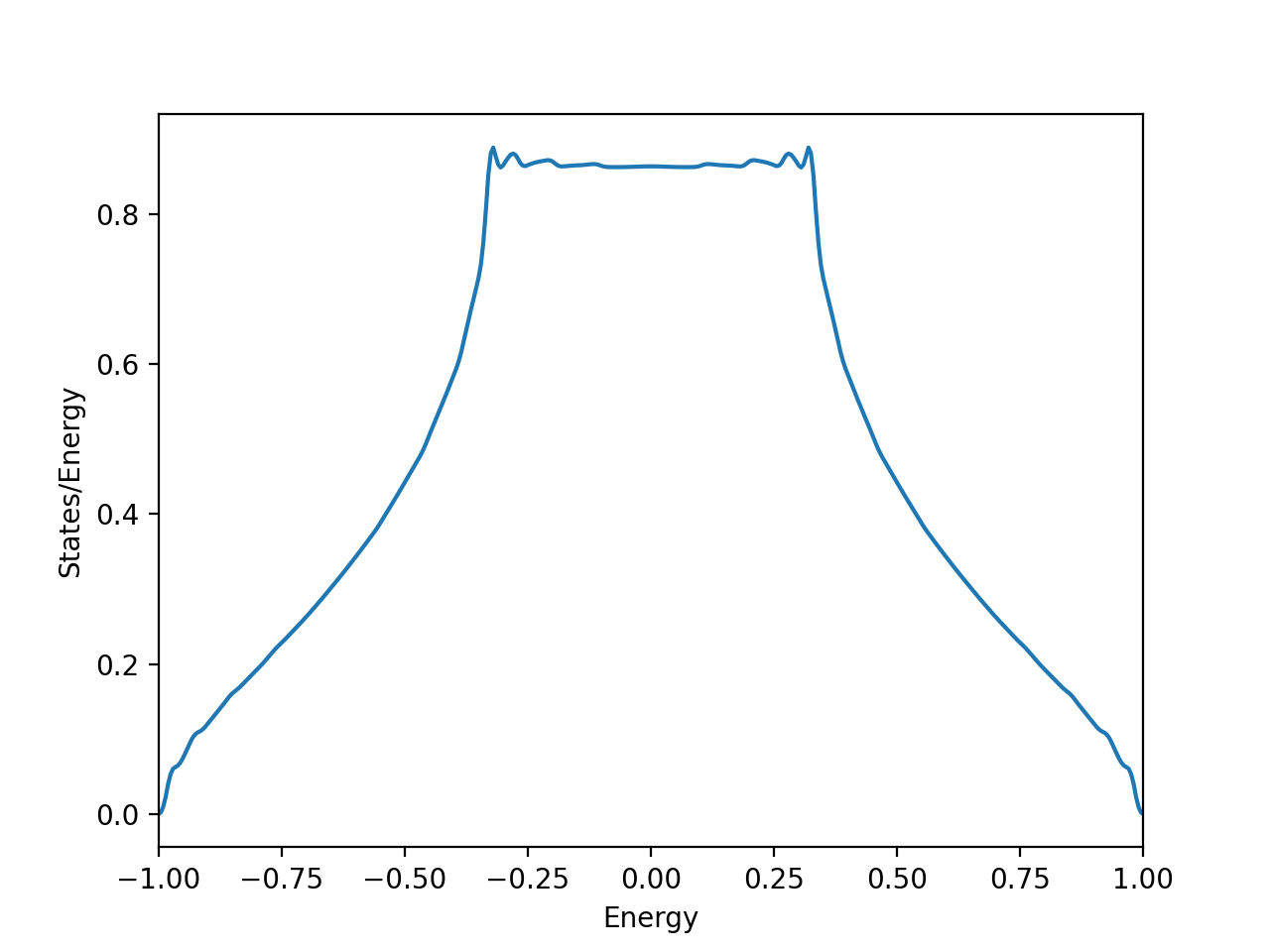
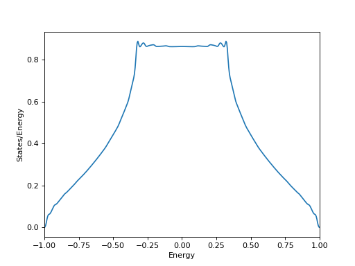
This will compute the DOS. The Fermi energy will be found for one electron per site.

(Source code, png, hires.png, pdf)

If we add a directive “-bands” or “bands=t” then the bands will be compute. Also, the program will make a file called “plt_bands.gr” which gracey.py can read and make a nice picture of the bands. If we run “gracey.py -i plt_bands.gr”, you will see the following:

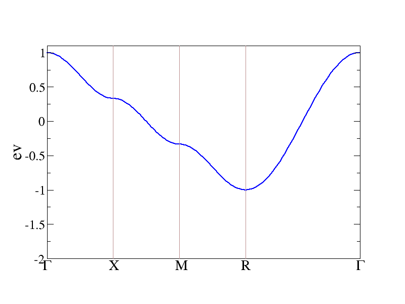
The bands of the Hubbard model on a cubic lattice computed using the tetrahedron method.

Now that we know how to explore the one-electron aspects of the real-space Hamiltonian, we will move on to include the effects of electron interactions. Let us compute the energy of the Hubbard model as a function of the on-site Coulomb repulsion . Let us begin by assuming that the energy of our Hubbard model is zero for . The energy of the model for and a finite will be for the non-spin-polarized case and for the spin polarized ferromagnetic case. Now, if we turn on a Hopping , the energy for the non-interacting case will be the first-moment of the filled portion of the DOS picture above. Accounting for the fact that we have two spins, we will get an energy of . For the NSP case, the energy would simply be . This will be an excellent approximation to the true energy when U is small as we will be in the perturbative regime.

What about when we do unrestricted Hartree-Fock? At sufficiently large U the system will choose to depopulate one of the spin channels to avoid the strong U. Let us go about computing the energy as a function of U. First let us run a single Hartree-Fock calculation. This may be done as follows:

tb_tools.py dens=1.0 ham=rham.py nk=20 pos=poscar tdos=t pg=oh nspin=2 U=4 ncor=1 -hf

You have to tell it a number of things. There must be two spins to do HF, we tell the code to do HF (ie. -hf or hf=t), and we declare that the number of correlated spatial orbitals is ncor=1. This code is general enough to handle uncorrelated states as well, but in this case there is just one state and it is correlated. Here is what the resulting DOS would look like for this case.

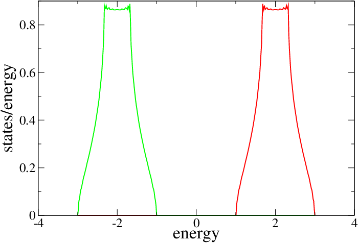
DOS of the Hubbard model on a cubic lattice for U=4 solved with Hartree-Fock. The system is clearly a ferromagnetic insulator.

Because we are dealing with an object oriented code, it is easier to write a simple program to do this as opposed to running tb_tools.py for different values of U and collecting the results (though this would be fine too). This can be done as follows:

from tb_tools import e_hamiltonian as hamiltonian
from numpy import arange

ham=hamiltonian('poscar','rham.py',dens=1.0,nk=20,pg='oh',nspin=2,ncor=1,U=2)

OUT=open('energy_vs_u.out','w')
for u in arange(0,2.05,0.1):
  ham.U=u
  ham.hartree_fock()
  OUT.write("%.4f %.6f %.6f\n"%(u,ham.energy,sum(ham.dm_sp)))

We can then plot the energy vs U, and we can even make the color of the point represent the spin. Gracey.py will plot this easily in contour mode as long as the color is given as a number between 100 and 200, so I use jkawk.py to renormalize the spin to this level.:

jkawk.py 'if l[0]<=2.:pp l[0],l[1],100+l[2]*100' energy_vs_u.out  | gracey.py -con pr=800,600 yl=Energy xl=U yr=-0.37,0.02

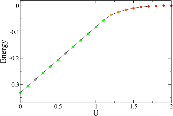
The energy of the Hubbard model on a cubic lattice as a function of U in unrestricted Hartree-Fock. Green means the moment is zero and red means the moment is 1 Bohr magneton (ie. fully polarized).

One can clearly see that the slope is 0.25, as indicated above in the analysis of the restricted HF. Once U becomes sufficiently large the system can gain energy by polarizing and sacrificing band energy at the expense of interaction energy. The system will become a fully polarized ferromagnetic insulator at U=2 and the energy will therefore be zero.

What if we want to compute the energy as a function of the density for a fixed U? This can be done with a similar procedure:

from tb_tools import e_hamiltonian as hamiltonian
from numpy import arange

OUT=open('energy_vs_dens.out','w')
for n in arange(0.1,1.05,0.1):
  ham=hamiltonian('poscar','rham.py',dens=n,nk=20,pg='oh',nspin=2,ncor=1,U=2)
  ham.hartree_fock()
  OUT.write("%.4f %.6f %.6f\n"%(n,ham.energy,sum(ham.dm_sp)))

One may also want to grab the non-interacting energy as a function of density:

from tb_tools import e_hamiltonian as hamiltonian
from numpy import arange

OUT=open('bandenergy_vs_dens.out','w')
for n in arange(0.1,1.05,0.1):
  ham=hamiltonian('poscar','rham.py',dens=n,nk=20,pg='oh',nspin=1,ncor=1)
  ham.compute_energy()
  OUT.write("%.4f %.6f 100\n"%(n,ham.energy))

The energy can now be plotted. As shown, in the limit of small density Hartree-Fock works well even though the U is rather large.

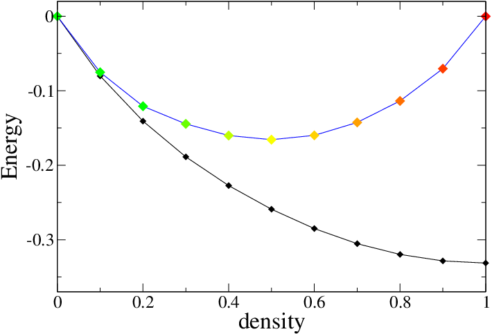
The energy of the Hubbard model on a cubic lattice as a function of density for U=2. The black curve is the non-interacting one, while the other is the unrestricted HF calculation. Once again, green means zero spin while red means fully polarized.

Periodic Anderson Model

To be continued…